In structural dynamics, geometry generally refers to the spatial layout of the measurements or analysis points. For example, in a modal test, we will generally have sensors distributed throughout the test article. The physical locations and orientations of those sensors represent the test geometry, and must be documented in order to map measurements taken during the test to physical locations on the test article. Similarly, in a finite element analysis, locations of nodes in the model will represent the analysis geometry.
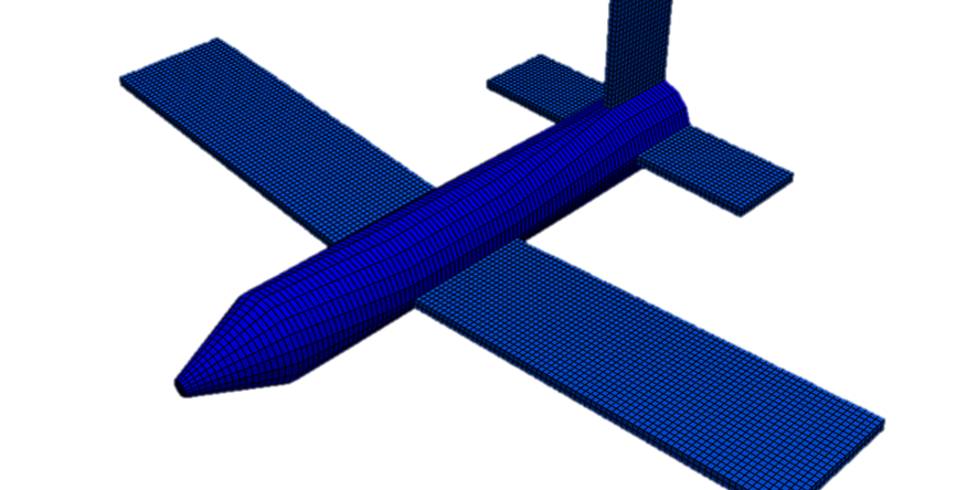
Figure 1:Geometry represents the spatial distribution of data points in a measurement or analysis.
This document will describe how geometry is defined and used in SDynPy. To start, a generic geometry will be created to demonstrate the process and describe the objects used. Subsequently, several example geometries of varying complexity will be created.
Let’s import SDynPy and start looking at geometry.
import sdynpy as sdpy
import numpy as np
SDynPy Geometry Objects
In SDynPy, the primary data type used to represent test or analysis geometry is the Geometry class defined in the sdynpy.geometry module. A typical SDynPy Geometry has four components:
Nodes: These are locations defined within the geometry and are represented by the
NodeArrayclass. Associated with each node is a unique identification number, a coordinate in 3D space, and references to the identification numbers of the coordinate systems used to define the nodes position and orientation.Coordinate Systems: These are coordinate systems that are used to define node positions and orientations and are represented by the
CoordinateSystemArrayclass. A simple geometry may have only one global coordinate used to define all node positions and orientations. A more complex geometry may have local coordinate systems defined relative to specific coordinates or measurements.Tracelines: These are lines drawn between nodes to enhance visualization of the geometry and are represented by the
TracelineArrayclass. Without visualization aids, the geometry would simply be a point cloud, which can be difficult to interpret, as it is not clear which points are in front of or behind other points.Elements: These are lines (e.g., bars), faces (e.g., triangles, quadrilaterals), or volumes (e.g., hexahedra, tetrahedra) drawn between nodes to enhance visualization of the geometry and are represented by the
ElementArrayclass. Without visualization aids, the geometry would simply be a point cloud, which can be difficult to interpret, as it is not clear which points are in front of or behind other points.
The general process to create a Geometry object is to first construct the desired components (NodeArray, CoordinateSystemArray, TracelineArray, and ElementArray) and then to pass them to the Geometry constructor.
Creating Geometry from Scratch
When performing a test, personnel instrumenting the test article should ideally be making measurements of the positions and orientations of each sensor. Similarly, for a finite element analysis positions of the nodes in the model can usually be extracted from the mesh file. These positions and orientations may be defined in many different ways depending on the test or analysis type. A cylindrical test article may most conveniently represent node positions in a cylindrical coordinate system, whereas test articles of other shapes may be better represented in cartesian or cylindrical coordinate systems. Orientation data may be represented in a multitude of formats: unit vectors of sensor directions, rotation matrices, quaternions, euler angles, etc. This information may be entered directly into a Python script to build the geometry, or it may come from an external file that must be read into Python. While SDynPy has several readers of common file formats which will be covered later in this section, the parsing of arbitrary file formats to extract desired information is outside the scope of this document. Therefore, for examples in this section, it will be assumed that the user can extract geometry data into the Python workspace in order to build these objects. This document will then show how that data can be packaged into a geometry object to represent the data.
Defining the Coordinate Systems in the Geometry
The first step to define a geometry is might intuitively be to define the nodes in the model; however, node positions are all defined with respect to some coordinate system, so the true first step should generally be to define the coordinate systems that the geometry will use. Simple geometries may only have one global coordinate system. More complex geometries may have an arbitrary number of coordinate systems defined.
Every node is assigned both a definition coordinate system and a displacement coordinate system. The definition coordinate system is the coordinate system in which the node positions are defined. The displacement coordinate system is the coordinate system in which the node deforms. The rationale for having two coordinate systems for each node is to allow the node to displace in a separate coordinate system from which it is defined. For example, a conical test article may have its nodes defined most conveniently in a cylindrical coordinate system with its radius from the cylindrical axis defined by the cone angle. However, if sensors are placed normal to the surface of the cone, they will not be aligned with the coordinate system used to define their location.
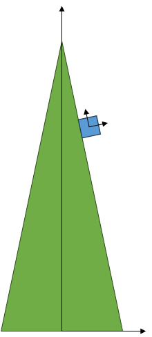
In the above photo, the test article is the green cone, and the blue square represents a sensor glued to the surface of the cone. The sensor will move in its own local coordinate system due to it being mounted obliquely to the part’s coordinate system, so it must have it’s own coordinate system defined. However, it may be significant additional effort to compute the position of the sensor in this local coordinate system, so it is allowable to define the sensor’s position in the global part coordinate system.
For simple geometries containing only a global coordinate system, the definition and displacement coordinate systems may be the same coordinate system.
For this initial demonstration, we will construct two coordinate systems, the first is a global cartesian coordinate system, the second will be a cylindrical coordinate system. Coordinate systems are defined in SDynPy using the CoordinateSystemArray object. Like most SdynpyArray objects, it has a helper function to allow easier definition, which is the same name as the object but in snake_case capitalization. In this case, the helper function is coordinate_system_array. We will define the coordinate systems unique identification numbers, as well as their type. SDynPy uses the integer 0 to represent a cartesian coordinate system, 1 to represent a cylindrical or polar coordinate system, and 2 to represent a spherical coordinate system. We also assign a name to each coordinate system, to make it more obvious what they represent. We could also assign a matrix representing the coordinate systems’ transformations from the global coordinate system; however, for simplicity at this point we will not do that. Later examples in this section will creating coordinate systems with custom matrices.
coordinate_systems = sdpy.coordinate_system_array(
    id = [1,2],
    cs_type = [0,1],
    name = ['Cartesian CS','Cylindrical CS'])
Let’s briefly explore the CoordinateSystemArray object before continuing. We can see by simply typing in the variable name into the terminal, we get a representation of the CoordinateSystemArray object.
coordinate_systems Index, ID, Name, Color, Type
(0,), 1, Cartesian CS, 1, Cartesian
(1,), 2, Cylindrical CS, 1, PolarTo see the data fields of a CoordinateSystemArray, we can use the fields property or examine its dtype for more information.
coordinate_systems.fields('id', 'name', 'color', 'cs_type', 'matrix')coordinate_systems.dtypedtype([('id', '<u8'), ('name', '<U40'), ('color', '<u2'), ('cs_type', '<u2'), ('matrix', '<f8', (4, 3))])To access one of the fields, we can simply use the field name like any other attribute of the object.
coordinate_systems.namearray(['Cartesian CS', 'Cylindrical CS'], dtype='<U40')These are the data that are stored within each coordinate system within a CoordinateSystemArray. Each coordinate system must have a unique positive integer identifier with which to reference it, and this is stored in the id field. Additionally, the name field allows a 40 character string to be defined that provides a name for the coordinate system. A color can also be assigned to a coordinate system; SDynPy does not actually apply colors to its coordinate system, but this can be defined to maintain consistency with Universal File Format Dataset 2420. Colors are defined using an integer from 0 to 15; see sdynpy.colors for the mapping of integers to colors. As stated previously, the coordinate system type is encoded as an integer in the cs_type field. Finally, the transformation matrix of the coordinate system is stored in the matrix field. Note in the dtype output, we see that the size of the matrix field is actually (4,3), meaning for each coordinate system in the CoordinateSystemArray is a 4 x 3 matrix consisting of a 3 x 3 rotation matrix above a 1 x 3 translation vector. See Coordinate System Transformations for more information on defining coordinate system matrices.
Note that when a field is defined containing a shape, the shape of this field will be appended to the shape of the object itself. For example, we have a shape (2,) CoordinateSystemArray:
coordinate_systems.shape(2,)If we look at the shape of the matrix field, we will see that the field is then (2,4,3):
coordinate_systems.matrix.shape(2, 4, 3)meaning that there is a (4,3) matrix for each of the (2,) coordinate systems.
Defining Nodes in the Geometry
With the coordinate systems defined, we will now define nodes in the geometry. Nodes are represented in SDynPy by the NodeArray object, which again is more conveniently constructed using the node_array function. Let’s construct a NodeArray for the nodes in the Cartesiean coordinate system. Depending on the complexity of the model, it may make sense to construct nodes in chunks and then combine them at the end, and we will show that here. One thing to keep in mind is that each node must have a unique identification number, so if combining nodes at a later point, ensure these identification numbers do not overlap.
We will start by defining the nodes for the cartesian section of the Geometry. We will simply make a 3 x 3 x 3 grid of points.
x_coordinates = [-1,0,1]
y_coordinates = [-1,0,1]
z_coordinates = [-3,-2,-1]
coordinates = []
for x in x_coordinates:
for y in y_coordinates:
for z in z_coordinates:
coordinates.append([x,y,z])
# Turn it into a NumPy array
coordinates = np.array(coordinates)
print(coordinates)[[-1 -1 -3]
[-1 -1 -2]
[-1 -1 -1]
[-1 0 -3]
[-1 0 -2]
[-1 0 -1]
[-1 1 -3]
[-1 1 -2]
[-1 1 -1]
[ 0 -1 -3]
[ 0 -1 -2]
[ 0 -1 -1]
[ 0 0 -3]
[ 0 0 -2]
[ 0 0 -1]
[ 0 1 -3]
[ 0 1 -2]
[ 0 1 -1]
[ 1 -1 -3]
[ 1 -1 -2]
[ 1 -1 -1]
[ 1 0 -3]
[ 1 0 -2]
[ 1 0 -1]
[ 1 1 -3]
[ 1 1 -2]
[ 1 1 -1]]
We see that our positions are a num_nodes by 3 array. Let’s also create the node identification numbers to go along with these points. To help us avoid numbering conflicts, we will start the cartesian nodes at 100.
node_ids_cartesian = [100+i for i,coordinate in enumerate(coordinates)]
print(node_ids_cartesian)[100, 101, 102, 103, 104, 105, 106, 107, 108, 109, 110, 111, 112, 113, 114, 115, 116, 117, 118, 119, 120, 121, 122, 123, 124, 125, 126]
Now let’s create the NodeArray:
cartesian_nodes = sdpy.node_array(
id = node_ids_cartesian,
coordinate = coordinates,
color = 1, # Blue
def_cs = 1, # Reference to our cartesian coordinate system ID Number
disp_cs = 1, # Reference to our cartesian coordiante system ID Number
)Now let’s do the same for our cylindrical coordinate system. We will start the node numbers for these nodes with 200.
r_coordinates = [1]
theta_coordinates = [0,45,90,135,180,215,270,335]
z_coordinates = [1,2,3]
coordinates = []
for r in r_coordinates:
for theta in theta_coordinates:
for z in z_coordinates:
coordinates.append([r,theta,z])
# Turn it into a NumPy array
coordinates = np.array(coordinates)
print(coordinates)[[ 1 0 1]
[ 1 0 2]
[ 1 0 3]
[ 1 45 1]
[ 1 45 2]
[ 1 45 3]
[ 1 90 1]
[ 1 90 2]
[ 1 90 3]
[ 1 135 1]
[ 1 135 2]
[ 1 135 3]
[ 1 180 1]
[ 1 180 2]
[ 1 180 3]
[ 1 215 1]
[ 1 215 2]
[ 1 215 3]
[ 1 270 1]
[ 1 270 2]
[ 1 270 3]
[ 1 335 1]
[ 1 335 2]
[ 1 335 3]]
node_ids_cylindrical = [200+i for i,coordinate in enumerate(coordinates)]
print(node_ids_cylindrical)[200, 201, 202, 203, 204, 205, 206, 207, 208, 209, 210, 211, 212, 213, 214, 215, 216, 217, 218, 219, 220, 221, 222, 223]
cylindrical_nodes = sdpy.node_array(
id = node_ids_cylindrical,
coordinate = coordinates,
color = 7, # Green
def_cs = 2, # Reference to our cylindrical coordinate system ID number
disp_cs = 2, # Reference to our cylindrical coordinate system ID number
)Recall that we can typically utilize NumPy functions with SdynpyArray objects. In this case, we will use np.concatenate to combine the two sets of nodes into one.
nodes = np.concatenate((cartesian_nodes, cylindrical_nodes))Before we go further, let’s also investigate the NodeArray object. Typing in the variable in the terminal will present a formatted node table for convenience.
nodes Index, ID, X, Y, Z, DefCS, DisCS
(0,), 100, -1.000, -1.000, -3.000, 1, 1
(1,), 101, -1.000, -1.000, -2.000, 1, 1
(2,), 102, -1.000, -1.000, -1.000, 1, 1
(3,), 103, -1.000, 0.000, -3.000, 1, 1
(4,), 104, -1.000, 0.000, -2.000, 1, 1
(5,), 105, -1.000, 0.000, -1.000, 1, 1
(6,), 106, -1.000, 1.000, -3.000, 1, 1
(7,), 107, -1.000, 1.000, -2.000, 1, 1
(8,), 108, -1.000, 1.000, -1.000, 1, 1
(9,), 109, 0.000, -1.000, -3.000, 1, 1
(10,), 110, 0.000, -1.000, -2.000, 1, 1
(11,), 111, 0.000, -1.000, -1.000, 1, 1
(12,), 112, 0.000, 0.000, -3.000, 1, 1
(13,), 113, 0.000, 0.000, -2.000, 1, 1
(14,), 114, 0.000, 0.000, -1.000, 1, 1
(15,), 115, 0.000, 1.000, -3.000, 1, 1
(16,), 116, 0.000, 1.000, -2.000, 1, 1
(17,), 117, 0.000, 1.000, -1.000, 1, 1
(18,), 118, 1.000, -1.000, -3.000, 1, 1
(19,), 119, 1.000, -1.000, -2.000, 1, 1
(20,), 120, 1.000, -1.000, -1.000, 1, 1
(21,), 121, 1.000, 0.000, -3.000, 1, 1
(22,), 122, 1.000, 0.000, -2.000, 1, 1
(23,), 123, 1.000, 0.000, -1.000, 1, 1
(24,), 124, 1.000, 1.000, -3.000, 1, 1
(25,), 125, 1.000, 1.000, -2.000, 1, 1
(26,), 126, 1.000, 1.000, -1.000, 1, 1
(27,), 200, 1.000, 0.000, 1.000, 2, 2
(28,), 201, 1.000, 0.000, 2.000, 2, 2
(29,), 202, 1.000, 0.000, 3.000, 2, 2
(30,), 203, 1.000, 45.000, 1.000, 2, 2
(31,), 204, 1.000, 45.000, 2.000, 2, 2
(32,), 205, 1.000, 45.000, 3.000, 2, 2
(33,), 206, 1.000, 90.000, 1.000, 2, 2
(34,), 207, 1.000, 90.000, 2.000, 2, 2
(35,), 208, 1.000, 90.000, 3.000, 2, 2
(36,), 209, 1.000, 135.000, 1.000, 2, 2
(37,), 210, 1.000, 135.000, 2.000, 2, 2
(38,), 211, 1.000, 135.000, 3.000, 2, 2
(39,), 212, 1.000, 180.000, 1.000, 2, 2
(40,), 213, 1.000, 180.000, 2.000, 2, 2
(41,), 214, 1.000, 180.000, 3.000, 2, 2
(42,), 215, 1.000, 215.000, 1.000, 2, 2
(43,), 216, 1.000, 215.000, 2.000, 2, 2
(44,), 217, 1.000, 215.000, 3.000, 2, 2
(45,), 218, 1.000, 270.000, 1.000, 2, 2
(46,), 219, 1.000, 270.000, 2.000, 2, 2
(47,), 220, 1.000, 270.000, 3.000, 2, 2
(48,), 221, 1.000, 335.000, 1.000, 2, 2
(49,), 222, 1.000, 335.000, 2.000, 2, 2
(50,), 223, 1.000, 335.000, 3.000, 2, 2To see the data fields of a NodeArray, we can use the fields property or examine its dtype for more information.
nodes.fields('id', 'coordinate', 'color', 'def_cs', 'disp_cs')nodes.dtypedtype([('id', '<u8'), ('coordinate', '<f8', (3,)), ('color', '<u2'), ('def_cs', '<u8'), ('disp_cs', '<u8')])Similar to the CoordinateSystemArray, we see that the id field, which contains the node ID
number, is a 8-byte (64-bit) unsigned integer. The geometry.node.disp_cs
and geometry.node.def_cs arrays, which contain references to the
coordinate systems in which the node is defined and in which the node
displaces, respectively, are also this data type. The color
array, while still an unsigned integer, is only 2 bytes, or 16 bits, and again represents the color assigned to each node in the geometry. Finally,
the coordinate field, which contains the 3D position of the node
as defined in the def_cs coordinate system, consists of
8-byte (64-bit)
floating-point data, and also has a shape of (3,), which signifies there
are three values of the coordinate for each entry in the NodeArray. These extra dimensions of the field arrays are appended at the end of
dimension of the object itself. For example, if we compare the shape of the NodeArray array
and its coordinate field, we will see that the shapes are
identical except for the appending of the length-3 extra dimension on the
latter array.
nodes.shape(51,)nodes.coordinate.shape(51, 3)Again, this means that there are three coordinates for each of the 51 nodes in our NodeArray.
Creating a Geometry
With a NodeArray and a CoordinateSystemArray defined, we now have the minimum dataset required to create a Geometry object. We could also create an ElementArray and a TracelineArray prior to constructing the Geometry; however, since these latter types are used only for visualization, it may be useful to first construct and plot the Geometry to understand which nodes should be connected using elements or lines.
We construct a Geometry object using its constructor directly. Note that unlike NodeArray and CoordinateSystemArray, we generally do not work with collections of geometries like we work with collections of nodes or collections of coordinate systems. Therefore, the Geometry object is not a subclass of SdynpyArray, and we use its constructor directly rather than some helper function. Note that this does not preclude storing, for example, multiple Geometry objects in a list if the application requires it. However Geometry objects are not optimized for such operations like NodeArray or CoordinateSystemArray objects.
geometry = sdpy.Geometry(
node=nodes,
coordinate_system=coordinate_systems)If we type in the variable name, we get a representation of the Geometry object.
geometryNode
Index, ID, X, Y, Z, DefCS, DisCS
(0,), 100, -1.000, -1.000, -3.000, 1, 1
(1,), 101, -1.000, -1.000, -2.000, 1, 1
(2,), 102, -1.000, -1.000, -1.000, 1, 1
(3,), 103, -1.000, 0.000, -3.000, 1, 1
(4,), 104, -1.000, 0.000, -2.000, 1, 1
(5,), 105, -1.000, 0.000, -1.000, 1, 1
(6,), 106, -1.000, 1.000, -3.000, 1, 1
(7,), 107, -1.000, 1.000, -2.000, 1, 1
(8,), 108, -1.000, 1.000, -1.000, 1, 1
(9,), 109, 0.000, -1.000, -3.000, 1, 1
(10,), 110, 0.000, -1.000, -2.000, 1, 1
(11,), 111, 0.000, -1.000, -1.000, 1, 1
(12,), 112, 0.000, 0.000, -3.000, 1, 1
(13,), 113, 0.000, 0.000, -2.000, 1, 1
(14,), 114, 0.000, 0.000, -1.000, 1, 1
(15,), 115, 0.000, 1.000, -3.000, 1, 1
(16,), 116, 0.000, 1.000, -2.000, 1, 1
(17,), 117, 0.000, 1.000, -1.000, 1, 1
(18,), 118, 1.000, -1.000, -3.000, 1, 1
(19,), 119, 1.000, -1.000, -2.000, 1, 1
(20,), 120, 1.000, -1.000, -1.000, 1, 1
(21,), 121, 1.000, 0.000, -3.000, 1, 1
(22,), 122, 1.000, 0.000, -2.000, 1, 1
(23,), 123, 1.000, 0.000, -1.000, 1, 1
(24,), 124, 1.000, 1.000, -3.000, 1, 1
(25,), 125, 1.000, 1.000, -2.000, 1, 1
(26,), 126, 1.000, 1.000, -1.000, 1, 1
(27,), 200, 1.000, 0.000, 1.000, 2, 2
(28,), 201, 1.000, 0.000, 2.000, 2, 2
(29,), 202, 1.000, 0.000, 3.000, 2, 2
(30,), 203, 1.000, 45.000, 1.000, 2, 2
(31,), 204, 1.000, 45.000, 2.000, 2, 2
(32,), 205, 1.000, 45.000, 3.000, 2, 2
(33,), 206, 1.000, 90.000, 1.000, 2, 2
(34,), 207, 1.000, 90.000, 2.000, 2, 2
(35,), 208, 1.000, 90.000, 3.000, 2, 2
(36,), 209, 1.000, 135.000, 1.000, 2, 2
(37,), 210, 1.000, 135.000, 2.000, 2, 2
(38,), 211, 1.000, 135.000, 3.000, 2, 2
(39,), 212, 1.000, 180.000, 1.000, 2, 2
(40,), 213, 1.000, 180.000, 2.000, 2, 2
(41,), 214, 1.000, 180.000, 3.000, 2, 2
(42,), 215, 1.000, 215.000, 1.000, 2, 2
(43,), 216, 1.000, 215.000, 2.000, 2, 2
(44,), 217, 1.000, 215.000, 3.000, 2, 2
(45,), 218, 1.000, 270.000, 1.000, 2, 2
(46,), 219, 1.000, 270.000, 2.000, 2, 2
(47,), 220, 1.000, 270.000, 3.000, 2, 2
(48,), 221, 1.000, 335.000, 1.000, 2, 2
(49,), 222, 1.000, 335.000, 2.000, 2, 2
(50,), 223, 1.000, 335.000, 3.000, 2, 2
Coordinate_system
   Index,     ID,                 Name, Color,       Type
    (0,),      1,         Cartesian CS,     1,  Cartesian
    (1,),      2,       Cylindrical CS,     1,      Polar
Traceline
   Index,     ID,          Description, Color, # Nodes
----------- Empty -------------
Element
   Index,     ID, Type, Color, # Nodes
----------- Empty -------------Note that since the Geometry is not a SdynpyArray or numpy.ndarray, there are no fields or dtype. There are instead only regular attributes.
geometry.dtype---------------------------------------------------------------------------
AttributeError Traceback (most recent call last)
Cell In[23], line 1
----> 1 geometry.dtype
AttributeError: 'Geometry' object has no attribute 'dtype'We can access the main properties of the geometry using the node, coordinate_system, element, or traceline attributes.
geometry.node Index, ID, X, Y, Z, DefCS, DisCS
(0,), 100, -1.000, -1.000, -3.000, 1, 1
(1,), 101, -1.000, -1.000, -2.000, 1, 1
(2,), 102, -1.000, -1.000, -1.000, 1, 1
(3,), 103, -1.000, 0.000, -3.000, 1, 1
(4,), 104, -1.000, 0.000, -2.000, 1, 1
(5,), 105, -1.000, 0.000, -1.000, 1, 1
(6,), 106, -1.000, 1.000, -3.000, 1, 1
(7,), 107, -1.000, 1.000, -2.000, 1, 1
(8,), 108, -1.000, 1.000, -1.000, 1, 1
(9,), 109, 0.000, -1.000, -3.000, 1, 1
(10,), 110, 0.000, -1.000, -2.000, 1, 1
(11,), 111, 0.000, -1.000, -1.000, 1, 1
(12,), 112, 0.000, 0.000, -3.000, 1, 1
(13,), 113, 0.000, 0.000, -2.000, 1, 1
(14,), 114, 0.000, 0.000, -1.000, 1, 1
(15,), 115, 0.000, 1.000, -3.000, 1, 1
(16,), 116, 0.000, 1.000, -2.000, 1, 1
(17,), 117, 0.000, 1.000, -1.000, 1, 1
(18,), 118, 1.000, -1.000, -3.000, 1, 1
(19,), 119, 1.000, -1.000, -2.000, 1, 1
(20,), 120, 1.000, -1.000, -1.000, 1, 1
(21,), 121, 1.000, 0.000, -3.000, 1, 1
(22,), 122, 1.000, 0.000, -2.000, 1, 1
(23,), 123, 1.000, 0.000, -1.000, 1, 1
(24,), 124, 1.000, 1.000, -3.000, 1, 1
(25,), 125, 1.000, 1.000, -2.000, 1, 1
(26,), 126, 1.000, 1.000, -1.000, 1, 1
(27,), 200, 1.000, 0.000, 1.000, 2, 2
(28,), 201, 1.000, 0.000, 2.000, 2, 2
(29,), 202, 1.000, 0.000, 3.000, 2, 2
(30,), 203, 1.000, 45.000, 1.000, 2, 2
(31,), 204, 1.000, 45.000, 2.000, 2, 2
(32,), 205, 1.000, 45.000, 3.000, 2, 2
(33,), 206, 1.000, 90.000, 1.000, 2, 2
(34,), 207, 1.000, 90.000, 2.000, 2, 2
(35,), 208, 1.000, 90.000, 3.000, 2, 2
(36,), 209, 1.000, 135.000, 1.000, 2, 2
(37,), 210, 1.000, 135.000, 2.000, 2, 2
(38,), 211, 1.000, 135.000, 3.000, 2, 2
(39,), 212, 1.000, 180.000, 1.000, 2, 2
(40,), 213, 1.000, 180.000, 2.000, 2, 2
(41,), 214, 1.000, 180.000, 3.000, 2, 2
(42,), 215, 1.000, 215.000, 1.000, 2, 2
(43,), 216, 1.000, 215.000, 2.000, 2, 2
(44,), 217, 1.000, 215.000, 3.000, 2, 2
(45,), 218, 1.000, 270.000, 1.000, 2, 2
(46,), 219, 1.000, 270.000, 2.000, 2, 2
(47,), 220, 1.000, 270.000, 3.000, 2, 2
(48,), 221, 1.000, 335.000, 1.000, 2, 2
(49,), 222, 1.000, 335.000, 2.000, 2, 2
(50,), 223, 1.000, 335.000, 3.000, 2, 2geometry.coordinate_system Index, ID, Name, Color, Type
(0,), 1, Cartesian CS, 1, Cartesian
(1,), 2, Cylindrical CS, 1, Polargeometry.traceline Index, ID, Description, Color, # Nodes
----------- Empty -------------geometry.element Index, ID, Type, Color, # Nodes
----------- Empty -------------We see that because we have constructed our geometry with only nodes and coordinate systems, the element and traceline fields are currently empty.
Since Geometry objects represent the spatial distribution of measurement or analysis points in a test or analysis, probably the most common thing to do with a geometry is to plot it.
geometry.plot(label_nodes=True);
This will bring up an interactive window in which the geometry can be rotated, panned, zoomed, or otherwise interacted with. There are numerous plotting options to supply to the Geometry method (see e.g. label_nodes in the previous commant). However, as the geometry currently stands, it is rather hard to interpret due to the lack of elements or lines connecting the nodes. It is simply a point-cloud currently, so many of the 3D cues that enable our brain to interpret a 2D image as a 3D scene are missing. We should presently add in those cues to allow us to easier interpret the geometry.
Adding Tracelines
Tracelines are lines that connect nodes in the Geometry to aid in visualization. There are two approaches to creating tracelines in the model. The first approach is to call the Geometry method to add tracelines one-by-one. The second approach is to construct a Geometry.plot explicitly and then assign it to Geometry.traceline (alternatively, one could pass it to the traceline argument of the Geometry.add_traceline constructor when initially creating the TracelineArray object). Given that we often would like to be looking at our Geometry object when figuring out which nodes to connect with a traceline, the former approach is usually the most straightforward, though there are case where the latter may be preferred, for instance when there is a pattern in the node numbers that can be exploited.
In this case, we will add tracelines to the cartesian portion of the model. SDynPy uses the convention that a 0 in the traceline connectivity array means to “pick up the pen” and will mean that there will be a gap in the line at that position.
geometry.add_traceline(
    connectivity = [100,103,106,115,124,121,118,109,100,0, # 0 means pick up the pen
                    101,104,107,116,125,122,119,110,101,0, # 0 means pick up the pen
                    102,105,108,117,126,123,120,111,102],
    id = 1,
    color = 1, # Blue
    description = 'Lines in the XY Plane',
    )
Note that when we call the Geometry.add_traceline method, we can explicitly assign an identification number with the id argument. If we don’t, SDynPy will automatically assign a unique identifier to the traceline that is one larger than the last largest identification number to avoid conflicts.
geometry.add_traceline(
    connectivity = [120,123,126,125,124,121,118,119,120,0, # 0 means pick up the pen
                    111,114,117,116,115,112,109,110,111,0, # 0 means pick up the pen
                    102,105,108,107,106,103,100,101,102],
    # We didn't explicitly add an id number here.
    color = 2, # Light Blue
    description = 'Lines in the YZ Plane',
    )
geometry.add_traceline(
connectivity = [126,117,108,107,106,115,124,125,126,0, # 0 means pick up the pen
123,114,105,104,103,112,121,122,123,0, # 0 means pick up the pen
120,111,102,101,100,109,118,119,120],
# We didn't explicitly add an id number here.
color = 3, # Gray Blue
description = 'Lines in the XZ Plane',
)Now if we plot the geometry, we can see that the added lines help with the interpretation of the cartesian portion of the geometry.
geometry.plot(label_nodes=True,line_width=2);
Let’s look at what the traceline attribute to see what we’ve added to the Geometry.
geometry.traceline Index, ID, Description, Color, # Nodes
(0,), 1, Lines in the XY Plane, 1, 29
(1,), 2, Lines in the YZ Plane, 2, 29
(2,), 3, Lines in the XZ Plane, 3, 29Geometry.traceline gives a TracelineArray object that contains the traceline definitions. We can again look at its fields or dtype.
geometry.traceline.fields('id', 'color', 'description', 'connectivity')geometry.traceline.dtypedtype([('id', '<u8'), ('color', '<u2'), ('description', '<U40'), ('connectivity', 'O')])Similarly to the other geometry objects,
TracelineArray objects
have id and color. The description field stores a name or description of each item in
the TracelineArray as
a string with less than 40 characters. Finally, the traceline
connectivity field is stored as an object array, where each entry in the
array is a NumPy ndarray with length equal to the number of nodes
in the traceline. This construction is necessary as each traceline might have a
different number of nodes, so a single array of fixed size is not possible.
geometry.traceline.connectivityarray([array([100, 103, 106, 115, 124, 121, 118, 109, 100, 0, 101, 104, 107,
116, 125, 122, 119, 110, 101, 0, 102, 105, 108, 117, 126, 123,
120, 111, 102], dtype=uint32) ,
array([120, 123, 126, 125, 124, 121, 118, 119, 120, 0, 111, 114, 117,
116, 115, 112, 109, 110, 111, 0, 102, 105, 108, 107, 106, 103,
100, 101, 102], dtype=uint32) ,
array([126, 117, 108, 107, 106, 115, 124, 125, 126, 0, 123, 114, 105,
104, 103, 112, 121, 122, 123, 0, 120, 111, 102, 101, 100, 109,
118, 119, 120], dtype=uint32) ],
dtype=object)Note that due to how object arrays are used in NumPy, investigating the
shape of the connectivity field will not immediately tell the user how many
nodes are in each connectivity array, but will rather just return the shape of
the TracelineArray
itself (note the dtype definition previously, where the connectivity field
has no additional shape associated with it).
geometry.traceline.shape(3,)geometry.traceline.connectivity.shape(3,)However, if we actually index into a single connectivity array, we can then see how big it is.
geometry.traceline.connectivity[0].shape(29,)Alternatively to the Geometry.add_traceline method, we could have constructed a TracelineArray explicitly and then used it in the construction of the Geometry or assigned it to the Geometry.traceline attribute. Like other SdynpyArray objects, there is a traceline_array function to help us construct the object.
# Extract items from the geometry to show how we can
# explicitly construct a traceline array
id_numbers = geometry.traceline.id
colors = geometry.traceline.color
descriptions = geometry.traceline.description
connectivity = geometry.traceline.connectivity

# Construct the TracelineArray
tracelines = sdpy.traceline_array(
    id = id_numbers,
    color = colors,
    description = descriptions,
    connectivity = connectivity)

tracelines
Index, ID, Description, Color, # Nodes
(0,), 1, Lines in the XY Plane, 1, 29
(1,), 2, Lines in the YZ Plane, 2, 29
(2,), 3, Lines in the XZ Plane, 3, 29We could then assign them to our geometry using the traceline attribute.
geometry.traceline = tracelinesOr if we knew the tracelines ahead of time, we could use them in the construction of the geometry directly.
geometry = sdpy.Geometry(
    node = nodes,
    coordinate_system = coordinate_systems,
    traceline = tracelines)
Adding Elements
The last portion of the geometry is elements. As opposed to a traceline, which can only connect between two nodes, elements can connect from three nodes in a triangle up to 20+ nodes in a hexahedral element. Elements in SDynPy follow closely the definition in Universal File Format Dataset 2412.
Because elements of different types may have the same number of nodes (e.g. a 4-node element could be a quadrilateral or a tetrahedral element), the type of each element must be explicitly defined. The element types used by SDynPy can be found in the sdpy.geometry._element_types attribute, and are encoded by an integer.
sdpy.geometry._element_types{11: 'Rod',
21: 'Linear beam',
22: 'Tapered beam',
23: 'Curved beam',
24: 'Parabolic beam',
31: 'Straight pipe',
32: 'Curved pipe',
41: 'Plane Stress Linear Triangle',
42: 'Plane Stress Parabolic Triangle',
43: 'Plane Stress Cubic Triangle',
44: 'Plane Stress Linear Quadrilateral',
45: 'Plane Stress Parabolic Quadrilateral',
46: 'Plane Strain Cubic Quadrilateral',
51: 'Plane Strain Linear Triangle',
52: 'Plane Strain Parabolic Triangle',
53: 'Plane Strain Cubic Triangle',
54: 'Plane Strain Linear Quadrilateral',
55: 'Plane Strain Parabolic Quadrilateral',
56: 'Plane Strain Cubic Quadrilateral',
61: 'Plate Linear Triangle',
62: 'Plate Parabolic Triangle',
63: 'Plate Cubic Triangle',
64: 'Plate Linear Quadrilateral',
65: 'Plate Parabolic Quadrilateral',
66: 'Plate Cubic Quadrilateral',
71: 'Membrane Linear Quadrilateral',
72: 'Membrane Parabolic Triangle',
73: 'Membrane Cubic Triangle',
74: 'Membrane Linear Triangle',
75: 'Membrane Parabolic Quadrilateral',
76: 'Membrane Cubic Quadrilateral',
81: 'Axisymetric Solid Linear Triangle',
82: 'Axisymetric Solid Parabolic Triangle',
84: 'Axisymetric Solid Linear Quadrilateral',
85: 'Axisymetric Solid Parabolic Quadrilateral',
91: 'Thin Shell Linear Triangle',
92: 'Thin Shell Parabolic Triangle',
93: 'Thin Shell Cubic Triangle',
94: 'Thin Shell Linear Quadrilateral',
95: 'Thin Shell Parabolic Quadrilateral',
96: 'Thin Shell Cubic Quadrilateral',
101: 'Thick Shell Linear Wedge',
102: 'Thick Shell Parabolic Wedge',
103: 'Thick Shell Cubic Wedge',
104: 'Thick Shell Linear Brick',
105: 'Thick Shell Parabolic Brick',
106: 'Thick Shell Cubic Brick',
111: 'Solid Linear Tetrahedron',
112: 'Solid Linear Wedge',
113: 'Solid Parabolic Wedge',
114: 'Solid Cubic Wedge',
115: 'Solid Linear Brick',
116: 'Solid Parabolic Brick',
117: 'Solid Cubic Brick',
118: 'Solid Parabolic Tetrahedron',
121: 'Rigid Bar',
122: 'Rigid Element',
136: 'Node To Node Translational Spring',
137: 'Node To Node Rotational Spring',
138: 'Node To Ground Translational Spring',
139: 'Node To Ground Rotational Spring',
141: 'Node To Node Damper',
142: 'Node To Gound Damper',
151: 'Node To Node Gap',
152: 'Node To Ground Gap',
161: 'Lumped Mass',
171: 'Axisymetric Linear Shell',
172: 'Axisymetric Parabolic Shell',
181: 'Constraint',
191: 'Plastic Cold Runner',
192: 'Plastic Hot Runner',
193: 'Plastic Water Line',
194: 'Plastic Fountain',
195: 'Plastic Baffle',
196: 'Plastic Rod Heater',
201: 'Linear node-to-node interface',
202: 'Linear edge-to-edge interface',
203: 'Parabolic edge-to-edge interface',
204: 'Linear face-to-face interface',
208: 'Parabolic face-to-face interface',
212: 'Linear axisymmetric interface',
213: 'Parabolic axisymmetric interface',
221: 'Linear rigid surface',
222: 'Parabolic rigid surface',
231: 'Axisymetric linear rigid surface',
232: 'Axisymentric parabolic rigid surface'}Note that SDynPy’s elements are only used for visualization, therefore SDynPy makes no distinction between, e.g., elements 51, 61, 71, 81, and 91, which are all variants of a triangular element. SDynPy will simply draw a triangle connecting the three nodes for any of these element types.
SDynPy stores element data in the ElementArray object. Similar to adding tracelines, elements can be added via a Geometry.add_element method, or alternatively by explicitly constructing an ElementArray object and assigning it to the Geometry.element attribute or by using it in the Geometry constructor. Again, given that we often would like to be looking at our Geometry object when figuring out which nodes to connect with an element, the former approach is usually the most straightforward, though there are case where the latter may be preferred, for instance when there is a pattern in the node numbers that can be exploited.
For this example, we will add triangular elements on the top row, and quadrilateral elements on the bottom row.
# Two triangles to complete the top row
geometry.add_element(
    elem_type = 61, # Plate linear triangle
    connectivity = [222, 223, 201],
    # id = 1, # We could explicitly assign an element number
    color = 7) # Green
geometry.add_element(
    elem_type = 61, # Plate linear triangle
    connectivity = [223,201,202],
    color = 7) # Green
# One Quad for the bottom row
geometry.add_element(
    elem_type = 64, # Plate linear quad
    connectivity = [221,222,201,200],
    color = 7) # Green

# Given how the node numbers are assembled, we can for loop
# to fill in the rest of the top row.
for i in range(7):
    # Triangles
    geometry.add_element(
        elem_type = 61, # Plate linear triangle
        connectivity = [201+3*i, 202+3*i, 204+3*i],
        color = 7) # Green
    geometry.add_element(
        elem_type = 61, # Plate linear triangle
        connectivity = [202+3*i, 204+3*i, 205+3*i],
        color = 7) # Green
    # Quad
    geometry.add_element(
        elem_type = 64, # Plate linear quad
        connectivity = [200+i*3, 201+i*3, 204+i*3, 203+i*3],
        color = 7) # Green
With elements, more interesting plotting options are available to us.
geometry.plot(label_nodes = True, show_edges = True, line_width = 2,
              opacity = 0.75)
(<sdynpy.GeometryPlotter at 0x1f70e288dd0>,
PolyData (0x1f70dbfc460)
N Cells: 33
N Points: 51
N Strips: 0
X Bounds: -1.000e+00, 1.000e+00
Y Bounds: -1.000e+00, 1.000e+00
Z Bounds: -3.000e+00, 3.000e+00
N Arrays: 1,
PolyData (0x1f70dbfc7c0)
N Cells: 51
N Points: 51
N Strips: 0
X Bounds: -1.000e+00, 1.000e+00
Y Bounds: -1.000e+00, 1.000e+00
Z Bounds: -3.000e+00, 3.000e+00
N Arrays: 2,
None)
Let’s look at the Geometry.element attribute to see what we have added to the Geometry object.
geometry.element Index, ID, Type, Color, # Nodes
(0,), 1, 61, 7, 3
(1,), 2, 61, 7, 3
(2,), 3, 64, 7, 4
(3,), 4, 61, 7, 3
(4,), 5, 61, 7, 3
(5,), 6, 64, 7, 4
(6,), 7, 61, 7, 3
(7,), 8, 61, 7, 3
(8,), 9, 64, 7, 4
(9,), 10, 61, 7, 3
(10,), 11, 61, 7, 3
(11,), 12, 64, 7, 4
(12,), 13, 61, 7, 3
(13,), 14, 61, 7, 3
(14,), 15, 64, 7, 4
(15,), 16, 61, 7, 3
(16,), 17, 61, 7, 3
(17,), 18, 64, 7, 4
(18,), 19, 61, 7, 3
(19,), 20, 61, 7, 3
(20,), 21, 64, 7, 4
(21,), 22, 61, 7, 3
(22,), 23, 61, 7, 3
(23,), 24, 64, 7, 4Geometry.element gives an ElementArray object. We can look at its fields and dtype attributes to see the underlying data.
geometry.element.fields('id', 'type', 'color', 'connectivity')geometry.element.dtypedtype([('id', '<u8'), ('type', 'u1'), ('color', '<u2'), ('connectivity', 'O')])Similarly to the TracelineArray, there is an id field containing a unique identification number, a color field that specifies the color applied to the element, and a connectivity field stored in an object array, where each entry in the
array is a NumPy ndarray with length equal to the number of nodes
in the traceline. This construction is necessary as each element might have a
different number of nodes, so a single array of fixed size is not possible. The element_type field is also present to store the type of element encoded as an integer.
Note that due to how object arrays are used in NumPy, investigating the
shape of the connectivity field will not immediately tell the user how many
nodes are in each connectivity array, but will rather just return the shape of
the ElementArray
itself (note the dtype definition previously, where the connectivity field
has no additional shape associated with it).
geometry.element.shape(24,)geometry.element.connectivity.shape(24,)However, if we index into one of the element’s connectivity, we can see the number of nodes in that element.
geometry.element[0].connectivity.shape(3,)Alternatively to the add_element method, we could have constructed a ElementArray explicitly and then used it in the construction of the Geometry or assigned it to the Geometry.element attribute. Like other SdynpyArray objects, there is a element_array function to help us construct the object.
# Extract items from the geometry to show how we can
# explicitly construct a traceline array
id_numbers = geometry.element.id
colors = geometry.element.color
types = geometry.element.type
connectivity = geometry.element.connectivity

# Construct the TracelineArray
elements = sdpy.element_array(
    id = id_numbers,
    color = colors,
    type = types,
    connectivity = connectivity)

elements
Index, ID, Type, Color, # Nodes
(0,), 1, 61, 7, 3
(1,), 2, 61, 7, 3
(2,), 3, 64, 7, 4
(3,), 4, 61, 7, 3
(4,), 5, 61, 7, 3
(5,), 6, 64, 7, 4
(6,), 7, 61, 7, 3
(7,), 8, 61, 7, 3
(8,), 9, 64, 7, 4
(9,), 10, 61, 7, 3
(10,), 11, 61, 7, 3
(11,), 12, 64, 7, 4
(12,), 13, 61, 7, 3
(13,), 14, 61, 7, 3
(14,), 15, 64, 7, 4
(15,), 16, 61, 7, 3
(16,), 17, 61, 7, 3
(17,), 18, 64, 7, 4
(18,), 19, 61, 7, 3
(19,), 20, 61, 7, 3
(20,), 21, 64, 7, 4
(21,), 22, 61, 7, 3
(22,), 23, 61, 7, 3
(23,), 24, 64, 7, 4We could then assign the ElementArray explicitly to the geometry by assigning to the element attribute.
geometry.element = elementsAlternatively, we could have used an explicitly constructed ElementArray in the Geometry constructor.
geometry = sdpy.Geometry(
    node = nodes,
    coordinate_system = coordinate_systems,
    traceline = tracelines,
    element = elements)
Creating Geometry from an Excel File Template
As an alternative to constructing a Geometry object using only code, SDynPy also has the capability to read in geometry data from a formatted Excel workbook using the from_excel_template class method. To generate an empty Excel workbook in the correct format, one can use the write_excel_template static method.
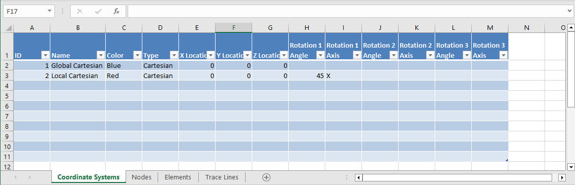
sdpy.Geometry.write_excel_template('geometry_template.xlsx')The template file contains a worksheet for the four main parts of the Geometry object; Coordinate Systems, Nodes, Elements, and Trace Lines. Many of the cells in the template contain data validation to ensure only appropriate content is entered.
Defining the Coordinate Systems
When defining the coordinate systems for a Geometry, the fields are much the same as when defining the items by code. The most significant different is that rather than defining the coordinate system transformation matrix by a 4 x 3 matrix, it is instead defined by a translation vector and a set of three rotations where the user can specify angle and axes. This could result in a more intuitive definition of rotated coordinate systems.
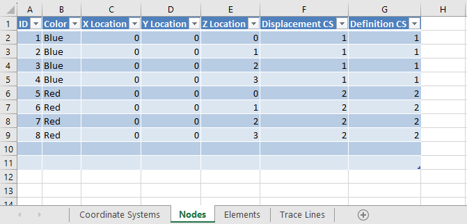
Defining the Nodes
Nodes are defined on the second sheet of the workbook. Users can manually enter identification number, color, location, and coordinate system information.
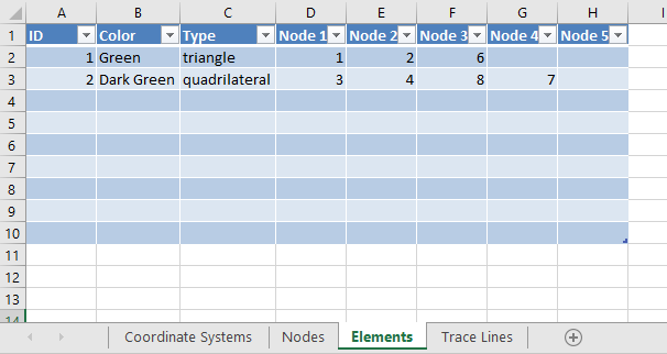
Defining the Elements
Elements are defined on the third sheet of the workbook. Identification number, type, color, and connectivity are all defined. In the workbook, the type is limited to beam, triangle, quadrilateral, or tetrahedron.
Defining the Tracelines
Tracelines can be defined on the last sheed of the workbook. Identification number, description, color, and connectivity are defined.
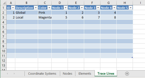
Loading the Geometry from the Completed Template
Once the template is filled out, the user can simply load the completed template into a Geometry object using the Geometry.from_excel_template class method.
geometry_from_excel = sdpy.Geometry.from_excel_template('geometry_template_completed.xlsx')
geometry_from_excel
Node
Index, ID, X, Y, Z, DefCS, DisCS
(0,), 1, 0.000, 0.000, 0.000, 1, 1
(1,), 2, 0.000, 0.000, 1.000, 1, 1
(2,), 3, 0.000, 0.000, 2.000, 1, 1
(3,), 4, 0.000, 0.000, 3.000, 1, 1
(4,), 5, 0.000, 0.000, 0.000, 2, 2
(5,), 6, 0.000, 0.000, 1.000, 2, 2
(6,), 7, 0.000, 0.000, 2.000, 2, 2
(7,), 8, 0.000, 0.000, 3.000, 2, 2
Coordinate_system
Index, ID, Name, Color, Type
(0,), 1, Global Cartesian, 1, Cartesian
(1,), 2, Local Cartesian, 11, Cartesian
Traceline
Index, ID, Description, Color, # Nodes
(0,), 1, Global, 14, 4
(1,), 2, Local, 12, 4
Element
Index, ID, Type, Color, # Nodes
(0,), 1, 41, 7, 3
(1,), 2, 44, 6, 4geometry_from_excel.plot();(<sdynpy.GeometryPlotter at 0x1f70e28ba40>,
PolyData (0x1f70e30b340)
N Cells: 4
N Points: 8
N Strips: 0
X Bounds: 0.000e+00, 0.000e+00
Y Bounds: -2.121e+00, 0.000e+00
Z Bounds: 0.000e+00, 3.000e+00
N Arrays: 1,
PolyData (0x1f70e30b4c0)
N Cells: 8
N Points: 8
N Strips: 0
X Bounds: 0.000e+00, 0.000e+00
Y Bounds: -2.121e+00, 0.000e+00
Z Bounds: 0.000e+00, 3.000e+00
N Arrays: 2,
None)
Reading and Writing Universal Files
A common storage mechanism for structural dynamics geometries is the Universal File Format. This file format consists of several dataset definitions. The datasets pertaining to Geometry are Datasets 82 (Tracelines), 2411 (Nodes), 2412 (Elements), and 2420 (Coordinate Systems). SDynPy’s geometry objects are modeled after these datasets and largely contain the same fields. Therefore it should come as no surprise that SDynPy’s geometry is largely compatible with the universal file format.
A geometry can be written to the universal file format by using its write_to_unv method.
geometry.write_to_unv('geometry.unv')This will write a file containing the following text (with the nodes in dataset 2411 and elements in dataset 2412 truncated for brevity).
    -1
  2420
         1

         1         0         1
Cartesian CS
   1.0000000000000000e+00   0.0000000000000000e+00   0.0000000000000000e+00
   0.0000000000000000e+00   1.0000000000000000e+00   0.0000000000000000e+00
   0.0000000000000000e+00   0.0000000000000000e+00   1.0000000000000000e+00
   0.0000000000000000e+00   0.0000000000000000e+00   0.0000000000000000e+00
         2         1         1
Spherical CS
   1.0000000000000000e+00   0.0000000000000000e+00   0.0000000000000000e+00
   0.0000000000000000e+00   1.0000000000000000e+00   0.0000000000000000e+00
   0.0000000000000000e+00   0.0000000000000000e+00   1.0000000000000000e+00
   0.0000000000000000e+00   0.0000000000000000e+00   0.0000000000000000e+00
    -1
    -1
  2411
       100         1         1         1
  -1.0000000000000000e+00  -1.0000000000000000e+00  -3.0000000000000000e+00
       101         1         1         1
  -1.0000000000000000e+00  -1.0000000000000000e+00  -2.0000000000000000e+00
. . .
       221         2         2         7
   1.0000000000000000e+00   3.3500000000000000e+02   1.0000000000000000e+00
       222         2         2         7
   1.0000000000000000e+00   3.3500000000000000e+02   2.0000000000000000e+00
       223         2         2         7
   1.0000000000000000e+00   3.3500000000000000e+02   3.0000000000000000e+00
    -1
    -1
  2412
         1        61         1         1         7         3
       222       223       201
         2        61         1         1         7         3
       223       201       202
         3        64         1         1         7         4
       221       222       201       200
         4        61         1         1         7         3
       201       202       204
. . .
        23        61         1         1         7         3
       220       222       223
        24        64         1         1         7         4
       218       219       222       221
    -1
    -1
    82
         1        29         1
Lines in the XY Plane
       100       103       106       115       124       121       118       109
       100         0       101       104       107       116       125       122
       119       110       101         0       102       105       108       117
       126       123       120       111       102
    -1
    -1
    82
         2        29         2
Lines in the YZ Plane
       120       123       126       125       124       121       118       119
       120         0       111       114       117       116       115       112
       109       110       111         0       102       105       108       107
       106       103       100       101       102
    -1
    -1
    82
         3        29         3
Lines in the XZ Plane
       126       117       108       107       106       115       124       125
       126         0       123       114       105       104       103       112
       121       122       123         0       120       111       102       101
       100       109       118       119       120
    -1
Similarly, a geometry can be read from a universal file. This can be done in multiple ways. If the universal file only contains geometry information, it can be easier to simply call the Geometry.load class method on the file to construct the Geometry object. The Geometry.load method will detect the .unv or .uff file extension and automatically pass the file to the SDynPy Universal File Format reader readunv. This will read the entire universal file and only keep datasets associated with the geometry. Note that the class method Geometry.load is also aliased to the module-level geometry.load function, so either is acceptable.
geometry = sdpy.geometry.load('geometry.unv')A secondary approach will call the readunv function explicitly. This approach is useful where the universal file may contain both geometry information and other types of information. Because Geometry.load will read the entire file, calling a separate function to read the remainder of the data will result in the entire file being read twice. Instead, the entire function can be read one time and the datasets parsed from the file can be passed to various functions to create SDynPy objects. A dictionary of dataset numbers and their contents is the output of readunv.
unv_dict = sdpy.unv.readunv('geometry.unv')
unv_dict
{2420: [Sdynpy_UFF_Dataset_2420<2 coordinate systems(s)>],
2411: [Sdynpy_UFF_Dataset_2411<51 node(s)>],
2412: [Sdynpy_UFF_Dataset_2414<24 element(s)>],
82: [Sdynpy_UFF_Dataset_82<traceline 1>,
Sdynpy_UFF_Dataset_82<traceline 2>,
Sdynpy_UFF_Dataset_82<traceline 3>]}This dictionary can be passed to the Geometry.from_unv class method to construct the geometry. Again, this class method is aliased to a module function geometry.from_unv for convenience.
geometry = sdpy.geometry.from_unv(unv_dict)Reading and Writing to NumPy Files
SDynPy does not have a native storage format for its data types. However, being built mostly on NumPy arrays, it is almost trivial to use NumPy format for storage. A Geometry object can be saved using its Geometry.save method. It will be written to a NumPy .npz file containing the nodes, elements, tracelines, and coordinate systems as data members.
geometry.save('geometry.npz')To load a Geometry object from this file, one can simply call the class method Geometry.load or its alias geometry.load, which will recognize the file extension and pass it to the NumPy loader.
geometry = sdpy.geometry.load('geometry.npz')Computing and Comparing Global Node Positions
Geometry in SDynPy is stored in the local coordinate system. For example, in the geometry we constructed, the coordinate for the cylindrical portion of the geometry is stored as (, , ) triples. However, it can be useful to quickly be able to compute the positions of these nodes in the global coordinate system, for example to compute the distance between two nodes. The global positions of specific nodes or all nodes can be computed using the Geometry method.
global_positions = geometry.global_node_coordinate()
global_positions
array([[-1.00000000e+00, -1.00000000e+00, -3.00000000e+00],
[-1.00000000e+00, -1.00000000e+00, -2.00000000e+00],
[-1.00000000e+00, -1.00000000e+00, -1.00000000e+00],
[-1.00000000e+00, 0.00000000e+00, -3.00000000e+00],
[-1.00000000e+00, 0.00000000e+00, -2.00000000e+00],
[-1.00000000e+00, 0.00000000e+00, -1.00000000e+00],
[-1.00000000e+00, 1.00000000e+00, -3.00000000e+00],
[-1.00000000e+00, 1.00000000e+00, -2.00000000e+00],
[-1.00000000e+00, 1.00000000e+00, -1.00000000e+00],
[ 0.00000000e+00, -1.00000000e+00, -3.00000000e+00],
[ 0.00000000e+00, -1.00000000e+00, -2.00000000e+00],
[ 0.00000000e+00, -1.00000000e+00, -1.00000000e+00],
[ 0.00000000e+00, 0.00000000e+00, -3.00000000e+00],
[ 0.00000000e+00, 0.00000000e+00, -2.00000000e+00],
[ 0.00000000e+00, 0.00000000e+00, -1.00000000e+00],
[ 0.00000000e+00, 1.00000000e+00, -3.00000000e+00],
[ 0.00000000e+00, 1.00000000e+00, -2.00000000e+00],
[ 0.00000000e+00, 1.00000000e+00, -1.00000000e+00],
[ 1.00000000e+00, -1.00000000e+00, -3.00000000e+00],
[ 1.00000000e+00, -1.00000000e+00, -2.00000000e+00],
[ 1.00000000e+00, -1.00000000e+00, -1.00000000e+00],
[ 1.00000000e+00, 0.00000000e+00, -3.00000000e+00],
[ 1.00000000e+00, 0.00000000e+00, -2.00000000e+00],
[ 1.00000000e+00, 0.00000000e+00, -1.00000000e+00],
[ 1.00000000e+00, 1.00000000e+00, -3.00000000e+00],
[ 1.00000000e+00, 1.00000000e+00, -2.00000000e+00],
[ 1.00000000e+00, 1.00000000e+00, -1.00000000e+00],
[ 1.00000000e+00, 0.00000000e+00, 1.00000000e+00],
[ 1.00000000e+00, 0.00000000e+00, 2.00000000e+00],
[ 1.00000000e+00, 0.00000000e+00, 3.00000000e+00],
[ 7.07106781e-01, 7.07106781e-01, 1.00000000e+00],
[ 7.07106781e-01, 7.07106781e-01, 2.00000000e+00],
[ 7.07106781e-01, 7.07106781e-01, 3.00000000e+00],
[ 6.12323400e-17, 1.00000000e+00, 1.00000000e+00],
[ 6.12323400e-17, 1.00000000e+00, 2.00000000e+00],
[ 6.12323400e-17, 1.00000000e+00, 3.00000000e+00],
[-7.07106781e-01, 7.07106781e-01, 1.00000000e+00],
[-7.07106781e-01, 7.07106781e-01, 2.00000000e+00],
[-7.07106781e-01, 7.07106781e-01, 3.00000000e+00],
[-1.00000000e+00, 1.22464680e-16, 1.00000000e+00],
[-1.00000000e+00, 1.22464680e-16, 2.00000000e+00],
[-1.00000000e+00, 1.22464680e-16, 3.00000000e+00],
[-8.19152044e-01, -5.73576436e-01, 1.00000000e+00],
[-8.19152044e-01, -5.73576436e-01, 2.00000000e+00],
[-8.19152044e-01, -5.73576436e-01, 3.00000000e+00],
[-1.83697020e-16, -1.00000000e+00, 1.00000000e+00],
[-1.83697020e-16, -1.00000000e+00, 2.00000000e+00],
[-1.83697020e-16, -1.00000000e+00, 3.00000000e+00],
[ 9.06307787e-01, -4.22618262e-01, 1.00000000e+00],
[ 9.06307787e-01, -4.22618262e-01, 2.00000000e+00],
[ 9.06307787e-01, -4.22618262e-01, 3.00000000e+00]])An optional node_ids argument can be passed to compute the positions of just specific nodes.
positions = geometry.global_node_coordinate(
    node_ids = [201,202,203,204])
positions
array([[1. , 0. , 2. ],
[1. , 0. , 3. ],
[0.70710678, 0.70710678, 1. ],
[0.70710678, 0.70710678, 2. ]])It may also be necessary to select nodes by global positions, meaning to find the node closest to a given position in space. For this, we can use the Geometry.node_by_global_position
points_to_find = np.array([[1,0,3],
                           [-1,0,3]])
closest_nodes = geometry.node_by_global_position(points_to_find)
closest_nodes
Index, ID, X, Y, Z, DefCS, DisCS
(0,), 202, 1.000, 0.000, 3.000, 2, 2
(1,), 214, 1.000, 180.000, 3.000, 2, 2And to get the closest nodes positions:
closest_node_positions = geometry.global_node_coordinate(closest_nodes.id)
closest_node_positions
array([[ 1.0000000e+00, 0.0000000e+00, 3.0000000e+00],
[-1.0000000e+00, 1.2246468e-16, 3.0000000e+00]])And the distances between the points:
distances = np.linalg.norm(points_to_find - closest_node_positions,axis=-1)
distances
array([0.0000000e+00, 1.2246468e-16])Coordinate System Transformations
The coordinate systems presented up until this point have all been aligned with the global cartesian coordinate system. SDynPy also offers the ability to create coordinate systems which are shifted or rotated with respect to the global coordinate system.
As stated previously, a CoordinateSystemArray has a field called matrix which is size 4 x 3, meaning each coordinate system defined in the Geometry contains a 4 x 3 transformation matrix. This defines the coordinate system’s rotation and translation with respect to the global coordinate system. The first three rows of the matrix field are defined as a 3 x 3 rotation matrix and the last row is defined as a 1 x 3 translation vector .
In SDynPy, a global coordinate can be transformed to a local coordinate via
Similarly, a local coordinate can be transformed to a global coordinate via
With this definition, the rows of the rotation matrix end up being the local , , and axes of the coordinate system represented in the global coordinate system.
Note that any cylindrical or spherical transformation be applied after this transformation matrix. For example, a cylindrical coordinate system with rotation matrix
will have its cylindrical axis pointing in the direction.
For the deflections, which are relative, the position component will cancel out. For example, to compute a global deflection from a local deflection , the equation is
Coordinate system transformations can be a relatively abstract concept, therefore SDynPy makes it easy to visualize coordinate systems to help users to understand if they have set theirs up correctly. The plot_coordinate method will plot a coordinate system triad at each node showing the displacement directions of that node as defined by its disp_cs coordinate system. This function will be described more in depth in Coordinates
geometry.plot_coordinate(arrow_scale = 0.025);<sdynpy.GeometryPlotter at 0x1f753765520>
In the plot, it is clear that the displacement directions of the cylindrical portion of the geometry follow the curvature of the cylinder, as that is their defined displacement coordinate system. The cartesian portion of the geometry follow the global coordinate system.
Reading and Writing to Exodus Files
Exodus is a file format used at Sandia National Laboratories and elsewhere for finite element analysis mesh definition and results storage. Because modal test and other structural dynamics datasets are often used to calibrate or validate models, it can be useful to bring the Exodus data and test data into SDynPy for comparison, or otherwise export the SDynPy data to an Exodus file for comparison using some other toolset.
Two types of exodus files exist in SDynPy. The first is the Exodus class, which is the more traditional Exodus interface. In this interface, data remains on disk until it is requested by calling a method of the Exodus class. The second is the ExodusInMemory class, which loads all data from disk and stores it in memory. In this class, data can be accessed via attributes.
In SDynPy, the Geometry is analogous to the node positions and element connectivity in the Exodus file. In the Exodus file, elements are stored in blocks which contain elements with the same element type, material, and other properties. Since SDynPy does not have the concept of element blocks, an element block is defined for each element type in the ElementArray. Similarly, a block is defined for each traceline in the TracelineArray.
To write a SDynPy geometry to an Exodus file, we will use the ExodusInMemory.from_sdynpy class method and pass it a Geometry object. This will create an ExodusInMemory object from the data in the Geometry object. Note that Exodus files generally do not store local coordinate system information, so all data is transformed to the global coordinate system prior to export. The ExodusInMemory.from_sdynpy class method can also accept results in the form of a ShapeArray or NDDataArray object via the displacement_data optional argument, which will be written to the Exodus file as nodal variables; however, in this example we will only supply the geometry data.
exo_in_memory = sdpy.ExodusInMemory.from_sdynpy(geometry)Once we have an ExodusInMemory object, we can write it to a file using ExodusInMemory.write_to_file. An optional clobber argument will overwrite an already existing file. If the file name exists and clobber=True is not specified, an error will occur.
exo_in_memory.write_to_file('geometry.exo',clobber=True)One the data is stored to an exodus file, it can be read in any number of Exodus readers. For example, the open-source software Paraview can read exodus files.
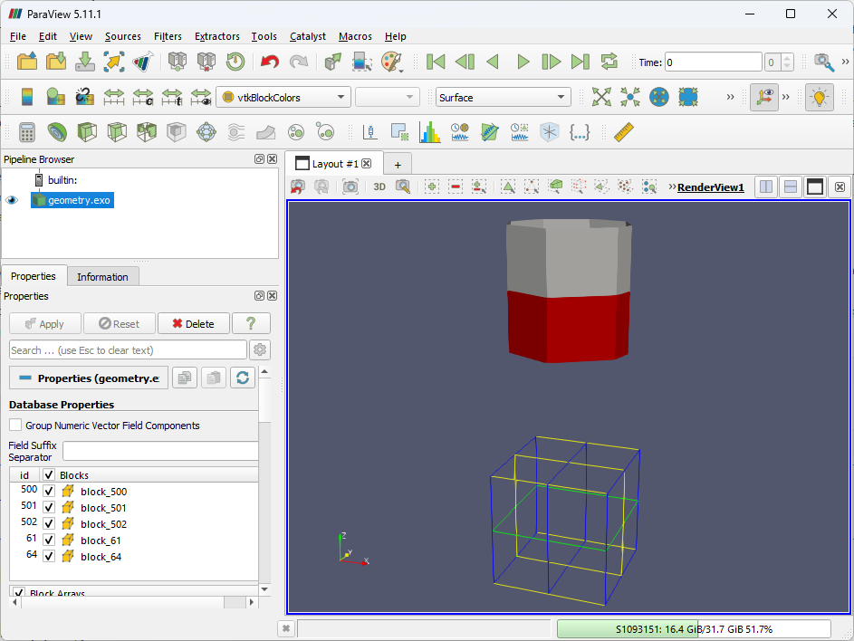
To read an Exodus file, we first use the Exodus class to open the file, then we can call Exodus.read_into_memory to generate an ExodusInMemory object if we desire. However, with the main goal to bring the Exodus data into a SDynPy geometry, we will generally use the Geometry.from_exodus class method to produce a SDynPy Geometry from either the Exodus or ExodusInMemory objects.
exo = sdpy.Exodus('geometry.exo')
exo
Exodus File at geometry.exo
1 Timesteps
51 Nodes
96 Elements
Blocks: 61, 64, 500, 501, 502
Node Variables: NodeColor
Element Variables: ElemColorgeometry_from_exodus = sdpy.Geometry.from_exodus(exo)
geometry_from_exodusNode
Index, ID, X, Y, Z, DefCS, DisCS
(0,), 100, -1.000, -1.000, -3.000, 1, 1
(1,), 101, -1.000, -1.000, -2.000, 1, 1
(2,), 102, -1.000, -1.000, -1.000, 1, 1
(3,), 103, -1.000, 0.000, -3.000, 1, 1
(4,), 104, -1.000, 0.000, -2.000, 1, 1
(5,), 105, -1.000, 0.000, -1.000, 1, 1
(6,), 106, -1.000, 1.000, -3.000, 1, 1
(7,), 107, -1.000, 1.000, -2.000, 1, 1
(8,), 108, -1.000, 1.000, -1.000, 1, 1
(9,), 109, 0.000, -1.000, -3.000, 1, 1
(10,), 110, 0.000, -1.000, -2.000, 1, 1
(11,), 111, 0.000, -1.000, -1.000, 1, 1
(12,), 112, 0.000, 0.000, -3.000, 1, 1
(13,), 113, 0.000, 0.000, -2.000, 1, 1
(14,), 114, 0.000, 0.000, -1.000, 1, 1
(15,), 115, 0.000, 1.000, -3.000, 1, 1
(16,), 116, 0.000, 1.000, -2.000, 1, 1
(17,), 117, 0.000, 1.000, -1.000, 1, 1
(18,), 118, 1.000, -1.000, -3.000, 1, 1
(19,), 119, 1.000, -1.000, -2.000, 1, 1
(20,), 120, 1.000, -1.000, -1.000, 1, 1
(21,), 121, 1.000, 0.000, -3.000, 1, 1
(22,), 122, 1.000, 0.000, -2.000, 1, 1
(23,), 123, 1.000, 0.000, -1.000, 1, 1
(24,), 124, 1.000, 1.000, -3.000, 1, 1
(25,), 125, 1.000, 1.000, -2.000, 1, 1
(26,), 126, 1.000, 1.000, -1.000, 1, 1
(27,), 200, 1.000, 0.000, 1.000, 1, 1
(28,), 201, 1.000, 0.000, 2.000, 1, 1
(29,), 202, 1.000, 0.000, 3.000, 1, 1
(30,), 203, 0.707, 0.707, 1.000, 1, 1
(31,), 204, 0.707, 0.707, 2.000, 1, 1
(32,), 205, 0.707, 0.707, 3.000, 1, 1
(33,), 206, 0.000, 1.000, 1.000, 1, 1
(34,), 207, 0.000, 1.000, 2.000, 1, 1
(35,), 208, 0.000, 1.000, 3.000, 1, 1
(36,), 209, -0.707, 0.707, 1.000, 1, 1
(37,), 210, -0.707, 0.707, 2.000, 1, 1
(38,), 211, -0.707, 0.707, 3.000, 1, 1
(39,), 212, -1.000, 0.000, 1.000, 1, 1
(40,), 213, -1.000, 0.000, 2.000, 1, 1
(41,), 214, -1.000, 0.000, 3.000, 1, 1
(42,), 215, -0.819, -0.574, 1.000, 1, 1
(43,), 216, -0.819, -0.574, 2.000, 1, 1
(44,), 217, -0.819, -0.574, 3.000, 1, 1
(45,), 218, -0.000, -1.000, 1.000, 1, 1
(46,), 219, -0.000, -1.000, 2.000, 1, 1
(47,), 220, -0.000, -1.000, 3.000, 1, 1
(48,), 221, 0.906, -0.423, 1.000, 1, 1
(49,), 222, 0.906, -0.423, 2.000, 1, 1
(50,), 223, 0.906, -0.423, 3.000, 1, 1
Coordinate_system
Index, ID, Name, Color, Type
(0,), 1, , 1, Cartesian
Traceline
Index, ID, Description, Color, # Nodes
----------- Empty -------------
Element
Index, ID, Type, Color, # Nodes
(0,), 1, 91, 1, 3
(1,), 2, 91, 1, 3
(2,), 3, 91, 1, 3
(3,), 4, 91, 1, 3
(4,), 5, 91, 1, 3
(5,), 6, 91, 1, 3
(6,), 7, 91, 1, 3
(7,), 8, 91, 1, 3
(8,), 9, 91, 1, 3
(9,), 10, 91, 1, 3
(10,), 11, 91, 1, 3
(11,), 12, 91, 1, 3
(12,), 13, 91, 1, 3
(13,), 14, 91, 1, 3
(14,), 15, 91, 1, 3
(15,), 16, 91, 1, 3
(16,), 17, 94, 2, 4
(17,), 18, 94, 2, 4
(18,), 19, 94, 2, 4
(19,), 20, 94, 2, 4
(20,), 21, 94, 2, 4
(21,), 22, 94, 2, 4
(22,), 23, 94, 2, 4
(23,), 24, 94, 2, 4
(24,), 25, 21, 3, 2
(25,), 26, 21, 3, 2
(26,), 27, 21, 3, 2
(27,), 28, 21, 3, 2
(28,), 29, 21, 3, 2
(29,), 30, 21, 3, 2
(30,), 31, 21, 3, 2
(31,), 32, 21, 3, 2
(32,), 33, 21, 3, 2
(33,), 34, 21, 3, 2
(34,), 35, 21, 3, 2
(35,), 36, 21, 3, 2
(36,), 37, 21, 3, 2
(37,), 38, 21, 3, 2
(38,), 39, 21, 3, 2
(39,), 40, 21, 3, 2
(40,), 41, 21, 3, 2
(41,), 42, 21, 3, 2
(42,), 43, 21, 3, 2
(43,), 44, 21, 3, 2
(44,), 45, 21, 3, 2
(45,), 46, 21, 3, 2
(46,), 47, 21, 3, 2
(47,), 48, 21, 3, 2
(48,), 49, 21, 4, 2
(49,), 50, 21, 4, 2
(50,), 51, 21, 4, 2
(51,), 52, 21, 4, 2
(52,), 53, 21, 4, 2
(53,), 54, 21, 4, 2
(54,), 55, 21, 4, 2
(55,), 56, 21, 4, 2
(56,), 57, 21, 4, 2
(57,), 58, 21, 4, 2
(58,), 59, 21, 4, 2
(59,), 60, 21, 4, 2
(60,), 61, 21, 4, 2
(61,), 62, 21, 4, 2
(62,), 63, 21, 4, 2
(63,), 64, 21, 4, 2
(64,), 65, 21, 4, 2
(65,), 66, 21, 4, 2
(66,), 67, 21, 4, 2
(67,), 68, 21, 4, 2
(68,), 69, 21, 4, 2
(69,), 70, 21, 4, 2
(70,), 71, 21, 4, 2
(71,), 72, 21, 4, 2
(72,), 73, 21, 5, 2
(73,), 74, 21, 5, 2
(74,), 75, 21, 5, 2
(75,), 76, 21, 5, 2
(76,), 77, 21, 5, 2
(77,), 78, 21, 5, 2
(78,), 79, 21, 5, 2
(79,), 80, 21, 5, 2
(80,), 81, 21, 5, 2
(81,), 82, 21, 5, 2
(82,), 83, 21, 5, 2
(83,), 84, 21, 5, 2
(84,), 85, 21, 5, 2
(85,), 86, 21, 5, 2
(86,), 87, 21, 5, 2
(87,), 88, 21, 5, 2
(88,), 89, 21, 5, 2
(89,), 90, 21, 5, 2
(90,), 91, 21, 5, 2
(91,), 92, 21, 5, 2
(92,), 93, 21, 5, 2
(93,), 94, 21, 5, 2
(94,), 95, 21, 5, 2
(95,), 96, 21, 5, 2It is important to note that SDynPy Geometry and Exodus files do not have the same feature set, and therefore we should not expect the Geometry we loaded from the Exodus file to be equivalent to the Geometry we originally saved to the Exodus file. For example, we see that the Geometry object that we loaded from the Exodus file only has a single coordinate system (the global coordinate system), and all nodes are defined in that coordinate system. Similarly, Exodus does not have the concept of tracelines, so the lines are stored as beam elements. Therefore, the Geometry loaded from the Exodus file has zero tracelines and several elements of type 21 (Linear Beam). Finally, the color information stored in the original Geometry is lost.
Geometry Reduction
Many times when working with geometries, it is useful to reduce the geometry to just a subset of the original geometry. For example, we may want to select only the cylindrical portion of the geometry we have created. However, such a reduction is more complicated than simply throwing away the nodes we do not want, because those nodes may be referenced by elements or tracelines. The safest way to remove a portion of a geometry is to use the Geometry.reduce method. This will automatically reduce to a Geometry object that contains only the specified nodes and only the elements and tracelines that contain those specified nodes.
Here we will select nodes. We recall that in our geometry, the cylinder nodes have -coordinate > 0 and the cube nodes have -coordinate < 0, so we can use that as a selection criterion. We are after the id field of each node that matches our criterion. Beware when working with NodeArray objects that the coordinate field is a local coordinate. This means that we can incorrectly select for nodes if we use position criteria that reference global positions while comparing to the local coordinate field. Unless you are sure that your geometry only has a single, global coordinate system, it is usually safer to use the global_node_coordinate method to ensure you are accessing the correct position.
global_positions = geometry.global_node_coordinate()
cylinder_nodes = geometry.node.id[global_positions[:,2] > 0]
cube_nodes = geometry.node.id[global_positions[:,2] < 0]
Once we have the nodes we want, we can pass the list of identification numbers to the Geometry.reduce method. This will not modify the Geometry in-place, but will rather return a copy of the Geometry object.
cylinder_geometry = geometry.reduce(cylinder_nodes)
cube_geometry = geometry.reduce(cube_nodes)
We can plot these to ensure the operations have been performed successfully.
cylinder_geometry.plot();(<sdynpy.GeometryPlotter at 0x1f753767020>,
PolyData (0x1f75376fee0)
N Cells: 24
N Points: 24
N Strips: 0
X Bounds: -1.000e+00, 1.000e+00
Y Bounds: -1.000e+00, 1.000e+00
Z Bounds: 1.000e+00, 3.000e+00
N Arrays: 1,
PolyData (0x1f75378c3a0)
N Cells: 24
N Points: 24
N Strips: 0
X Bounds: -1.000e+00, 1.000e+00
Y Bounds: -1.000e+00, 1.000e+00
Z Bounds: 1.000e+00, 3.000e+00
N Arrays: 2,
None)
cube_geometry.plot();(<sdynpy.GeometryPlotter at 0x1f753767260>,
PolyData (0x1f75378d180)
N Cells: 9
N Points: 27
N Strips: 0
X Bounds: -1.000e+00, 1.000e+00
Y Bounds: -1.000e+00, 1.000e+00
Z Bounds: -3.000e+00, -1.000e+00
N Arrays: 1,
PolyData (0x1f75378d4e0)
N Cells: 27
N Points: 27
N Strips: 0
X Bounds: -1.000e+00, 1.000e+00
Y Bounds: -1.000e+00, 1.000e+00
Z Bounds: -3.000e+00, -1.000e+00
N Arrays: 2,
None)
Combining Geometries
Similarly to reducing Geometry objects, there can be times where we want to combine geometry objects into a single object. SDynPy has two ways to do this. The first way is to simply add the two Geometry objects together. In this case, the NodeArray, CoordinateSystemArray, TracelineArray, and ElementArray objects from the respective Geometry objects will simply be concatenated together.
combined_geometry = cube_geometry + cylinder_geometryNote that SDynPy will check to ensure there aren’t conflicts between the Geometry objects. For example, if two nodes are labeled 100 but they have different data associated with them, SDynPy will throw an error.
# Make a copy of the cube geometry
cube_geometry_2 = cube_geometry.copy()
# Change some data associated with it
cube_geometry_2.node[0].color = 13
# Now try to add them together
cube_geometry+cube_geometry_2
---------------------------------------------------------------------------
ValueError Traceback (most recent call last)
Cell In[79], line 6
4 cube_geometry_2.node[0].color = 13
5 # Now try to add them together
----> 6 cube_geometry+cube_geometry_2
File ~\Documents\Local_Repositories\sdynpy\src\sdynpy\core\sdynpy_geometry.py:4788, in Geometry.__add__(self, geometry)
4786 equal_ids = getattr(self, field)(common_ids) == getattr(geometry, field)(common_ids)
4787 if not all(equal_ids):
-> 4788 raise ValueError('Both geometries contain {:} with ID {:} but they are not equivalent'.format(
4789 field, common_ids[~equal_ids]))
4790 self_ids = np.concatenate(
4791 (np.setdiff1d(getattr(self, field).id, getattr(geometry, field).id), common_ids))
4792 geometry_ids = np.setdiff1d(getattr(geometry, field).id, getattr(self, field).id)
ValueError: Both geometries contain node with ID [100] but they are not equivalentNote that if two items share the same identification number but they have identical underlying data, then the concatenation will succeed. The identical data between the two geometries will not be duplicated; only one copy will remain. This is useful when, for example, concatenating two geometries which both have a global coordinate system with identification number 1.
The second way to combine two geometries is to use the Geometry.overlay_geometries method. This method is typically used when two geometries from different sources are to be compared. Instead of combining the identification numbers of the items in the Geometry objects, it instead computes an offset value that gets applied to the identification numbers to ensure there are no conflicts. These offsets can be returned by the method as well by passing optional arguments.
overlaid_geometry,node_offset = sdpy.Geometry.overlay_geometries((cube_geometry,cylinder_geometry),return_node_id_offset=True)Comparing the combined_geometry from the concatenation and the overlaid_geometry from Geometry.overlay_geometries, we can see how the offset is applied. Recalling the original node numbers:
# Original cube nodes
cube_geometry.node
Index, ID, X, Y, Z, DefCS, DisCS
(0,), 100, -1.000, -1.000, -3.000, 1, 1
(1,), 101, -1.000, -1.000, -2.000, 1, 1
(2,), 102, -1.000, -1.000, -1.000, 1, 1
(3,), 103, -1.000, 0.000, -3.000, 1, 1
(4,), 104, -1.000, 0.000, -2.000, 1, 1
(5,), 105, -1.000, 0.000, -1.000, 1, 1
(6,), 106, -1.000, 1.000, -3.000, 1, 1
(7,), 107, -1.000, 1.000, -2.000, 1, 1
(8,), 108, -1.000, 1.000, -1.000, 1, 1
(9,), 109, 0.000, -1.000, -3.000, 1, 1
(10,), 110, 0.000, -1.000, -2.000, 1, 1
(11,), 111, 0.000, -1.000, -1.000, 1, 1
(12,), 112, 0.000, 0.000, -3.000, 1, 1
(13,), 113, 0.000, 0.000, -2.000, 1, 1
(14,), 114, 0.000, 0.000, -1.000, 1, 1
(15,), 115, 0.000, 1.000, -3.000, 1, 1
(16,), 116, 0.000, 1.000, -2.000, 1, 1
(17,), 117, 0.000, 1.000, -1.000, 1, 1
(18,), 118, 1.000, -1.000, -3.000, 1, 1
(19,), 119, 1.000, -1.000, -2.000, 1, 1
(20,), 120, 1.000, -1.000, -1.000, 1, 1
(21,), 121, 1.000, 0.000, -3.000, 1, 1
(22,), 122, 1.000, 0.000, -2.000, 1, 1
(23,), 123, 1.000, 0.000, -1.000, 1, 1
(24,), 124, 1.000, 1.000, -3.000, 1, 1
(25,), 125, 1.000, 1.000, -2.000, 1, 1
(26,), 126, 1.000, 1.000, -1.000, 1, 1# Original cylinder nodes
cylinder_geometry.node Index, ID, X, Y, Z, DefCS, DisCS
(0,), 200, 1.000, 0.000, 1.000, 2, 2
(1,), 201, 1.000, 0.000, 2.000, 2, 2
(2,), 202, 1.000, 0.000, 3.000, 2, 2
(3,), 203, 1.000, 45.000, 1.000, 2, 2
(4,), 204, 1.000, 45.000, 2.000, 2, 2
(5,), 205, 1.000, 45.000, 3.000, 2, 2
(6,), 206, 1.000, 90.000, 1.000, 2, 2
(7,), 207, 1.000, 90.000, 2.000, 2, 2
(8,), 208, 1.000, 90.000, 3.000, 2, 2
(9,), 209, 1.000, 135.000, 1.000, 2, 2
(10,), 210, 1.000, 135.000, 2.000, 2, 2
(11,), 211, 1.000, 135.000, 3.000, 2, 2
(12,), 212, 1.000, 180.000, 1.000, 2, 2
(13,), 213, 1.000, 180.000, 2.000, 2, 2
(14,), 214, 1.000, 180.000, 3.000, 2, 2
(15,), 215, 1.000, 215.000, 1.000, 2, 2
(16,), 216, 1.000, 215.000, 2.000, 2, 2
(17,), 217, 1.000, 215.000, 3.000, 2, 2
(18,), 218, 1.000, 270.000, 1.000, 2, 2
(19,), 219, 1.000, 270.000, 2.000, 2, 2
(20,), 220, 1.000, 270.000, 3.000, 2, 2
(21,), 221, 1.000, 335.000, 1.000, 2, 2
(22,), 222, 1.000, 335.000, 2.000, 2, 2
(23,), 223, 1.000, 335.000, 3.000, 2, 2We see that when we concatenate, those numbers are maintained.
# Combined nodes have identical IDs as the original geometries
combined_geometry.node
Index, ID, X, Y, Z, DefCS, DisCS
(0,), 100, -1.000, -1.000, -3.000, 1, 1
(1,), 101, -1.000, -1.000, -2.000, 1, 1
(2,), 102, -1.000, -1.000, -1.000, 1, 1
(3,), 103, -1.000, 0.000, -3.000, 1, 1
(4,), 104, -1.000, 0.000, -2.000, 1, 1
(5,), 105, -1.000, 0.000, -1.000, 1, 1
(6,), 106, -1.000, 1.000, -3.000, 1, 1
(7,), 107, -1.000, 1.000, -2.000, 1, 1
(8,), 108, -1.000, 1.000, -1.000, 1, 1
(9,), 109, 0.000, -1.000, -3.000, 1, 1
(10,), 110, 0.000, -1.000, -2.000, 1, 1
(11,), 111, 0.000, -1.000, -1.000, 1, 1
(12,), 112, 0.000, 0.000, -3.000, 1, 1
(13,), 113, 0.000, 0.000, -2.000, 1, 1
(14,), 114, 0.000, 0.000, -1.000, 1, 1
(15,), 115, 0.000, 1.000, -3.000, 1, 1
(16,), 116, 0.000, 1.000, -2.000, 1, 1
(17,), 117, 0.000, 1.000, -1.000, 1, 1
(18,), 118, 1.000, -1.000, -3.000, 1, 1
(19,), 119, 1.000, -1.000, -2.000, 1, 1
(20,), 120, 1.000, -1.000, -1.000, 1, 1
(21,), 121, 1.000, 0.000, -3.000, 1, 1
(22,), 122, 1.000, 0.000, -2.000, 1, 1
(23,), 123, 1.000, 0.000, -1.000, 1, 1
(24,), 124, 1.000, 1.000, -3.000, 1, 1
(25,), 125, 1.000, 1.000, -2.000, 1, 1
(26,), 126, 1.000, 1.000, -1.000, 1, 1
(27,), 200, 1.000, 0.000, 1.000, 2, 2
(28,), 201, 1.000, 0.000, 2.000, 2, 2
(29,), 202, 1.000, 0.000, 3.000, 2, 2
(30,), 203, 1.000, 45.000, 1.000, 2, 2
(31,), 204, 1.000, 45.000, 2.000, 2, 2
(32,), 205, 1.000, 45.000, 3.000, 2, 2
(33,), 206, 1.000, 90.000, 1.000, 2, 2
(34,), 207, 1.000, 90.000, 2.000, 2, 2
(35,), 208, 1.000, 90.000, 3.000, 2, 2
(36,), 209, 1.000, 135.000, 1.000, 2, 2
(37,), 210, 1.000, 135.000, 2.000, 2, 2
(38,), 211, 1.000, 135.000, 3.000, 2, 2
(39,), 212, 1.000, 180.000, 1.000, 2, 2
(40,), 213, 1.000, 180.000, 2.000, 2, 2
(41,), 214, 1.000, 180.000, 3.000, 2, 2
(42,), 215, 1.000, 215.000, 1.000, 2, 2
(43,), 216, 1.000, 215.000, 2.000, 2, 2
(44,), 217, 1.000, 215.000, 3.000, 2, 2
(45,), 218, 1.000, 270.000, 1.000, 2, 2
(46,), 219, 1.000, 270.000, 2.000, 2, 2
(47,), 220, 1.000, 270.000, 3.000, 2, 2
(48,), 221, 1.000, 335.000, 1.000, 2, 2
(49,), 222, 1.000, 335.000, 2.000, 2, 2
(50,), 223, 1.000, 335.000, 3.000, 2, 2However, when we overlay the geometries, an offset is applied.
node_offset1000SDynPy computed the offset of 1000, and will add 1*1000 to the first geometry, 2*1000 to the second geometry, etc. In this way, it can be ensured that no conflicts occur.
In the overlaid geometry, we see that the cube nodes start with 1000 and the cylinder nodes start with 2000.
overlaid_geometry.node Index, ID, X, Y, Z, DefCS, DisCS
(0,), 1100, -1.000, -1.000, -3.000, 11, 11
(1,), 1101, -1.000, -1.000, -2.000, 11, 11
(2,), 1102, -1.000, -1.000, -1.000, 11, 11
(3,), 1103, -1.000, 0.000, -3.000, 11, 11
(4,), 1104, -1.000, 0.000, -2.000, 11, 11
(5,), 1105, -1.000, 0.000, -1.000, 11, 11
(6,), 1106, -1.000, 1.000, -3.000, 11, 11
(7,), 1107, -1.000, 1.000, -2.000, 11, 11
(8,), 1108, -1.000, 1.000, -1.000, 11, 11
(9,), 1109, 0.000, -1.000, -3.000, 11, 11
(10,), 1110, 0.000, -1.000, -2.000, 11, 11
(11,), 1111, 0.000, -1.000, -1.000, 11, 11
(12,), 1112, 0.000, 0.000, -3.000, 11, 11
(13,), 1113, 0.000, 0.000, -2.000, 11, 11
(14,), 1114, 0.000, 0.000, -1.000, 11, 11
(15,), 1115, 0.000, 1.000, -3.000, 11, 11
(16,), 1116, 0.000, 1.000, -2.000, 11, 11
(17,), 1117, 0.000, 1.000, -1.000, 11, 11
(18,), 1118, 1.000, -1.000, -3.000, 11, 11
(19,), 1119, 1.000, -1.000, -2.000, 11, 11
(20,), 1120, 1.000, -1.000, -1.000, 11, 11
(21,), 1121, 1.000, 0.000, -3.000, 11, 11
(22,), 1122, 1.000, 0.000, -2.000, 11, 11
(23,), 1123, 1.000, 0.000, -1.000, 11, 11
(24,), 1124, 1.000, 1.000, -3.000, 11, 11
(25,), 1125, 1.000, 1.000, -2.000, 11, 11
(26,), 1126, 1.000, 1.000, -1.000, 11, 11
(27,), 2200, 1.000, 0.000, 1.000, 22, 22
(28,), 2201, 1.000, 0.000, 2.000, 22, 22
(29,), 2202, 1.000, 0.000, 3.000, 22, 22
(30,), 2203, 1.000, 45.000, 1.000, 22, 22
(31,), 2204, 1.000, 45.000, 2.000, 22, 22
(32,), 2205, 1.000, 45.000, 3.000, 22, 22
(33,), 2206, 1.000, 90.000, 1.000, 22, 22
(34,), 2207, 1.000, 90.000, 2.000, 22, 22
(35,), 2208, 1.000, 90.000, 3.000, 22, 22
(36,), 2209, 1.000, 135.000, 1.000, 22, 22
(37,), 2210, 1.000, 135.000, 2.000, 22, 22
(38,), 2211, 1.000, 135.000, 3.000, 22, 22
(39,), 2212, 1.000, 180.000, 1.000, 22, 22
(40,), 2213, 1.000, 180.000, 2.000, 22, 22
(41,), 2214, 1.000, 180.000, 3.000, 22, 22
(42,), 2215, 1.000, 215.000, 1.000, 22, 22
(43,), 2216, 1.000, 215.000, 2.000, 22, 22
(44,), 2217, 1.000, 215.000, 3.000, 22, 22
(45,), 2218, 1.000, 270.000, 1.000, 22, 22
(46,), 2219, 1.000, 270.000, 2.000, 22, 22
(47,), 2220, 1.000, 270.000, 3.000, 22, 22
(48,), 2221, 1.000, 335.000, 1.000, 22, 22
(49,), 2222, 1.000, 335.000, 2.000, 22, 22
(50,), 2223, 1.000, 335.000, 3.000, 22, 22Geometry Mapping
Many times in Structural Dynamics applications, we will want to compare two datasets. Perhaps a test is being compared to its equivalent simulation, or two simulations are compared to evaluate modeling assumptions. Regardless, these two datasets will very often not have compatible geometry. A test may have a few hundred sensors, whereas a finite element model may have a few million degrees of freedom. Regardless, we often wish to compare degrees of freedom, and for that reason, SDynPy defines an id_map object. The id_map object is essentially a vectorized dictionary that accepts an identification number and returns a new identification number that the first identification number is mapped to.
To show an example, let’s randomly generate some large numbers that we can pretend are node identification numbers from a finite element analysis.
finite_element_nodes = np.random.randint(10000, 99999, geometry.node.id.shape) # Create the same number as nodes in our geometry.
finite_element_nodes
array([11670, 28449, 98106, 20627, 23129, 21286, 74121, 66502, 31148,
72041, 13563, 79736, 16396, 59804, 38123, 27568, 97885, 29102,
71300, 22011, 62136, 52105, 74824, 99876, 80960, 98549, 18948,
45608, 75611, 66314, 74172, 71075, 13705, 46925, 14813, 22640,
63466, 94966, 18798, 84972, 71707, 77675, 20645, 68801, 87053,
34258, 78930, 56828, 47752, 35918, 54862], dtype=int32)To set up this map, we then supply the nodes we are mapping from (e.g. our geometry’s nodes) and the nodes we are mapping to (e.g. these fake finite element node numbers).
node_id_map = sdpy.id_map(
    from_ids = geometry.node.id,
    to_ids = finite_element_nodes)
To explicitly map the nodes, we can then call the Geometry.map_ids method, and pass it this id_map object.
mapped_geometry = geometry.map_ids(
    node_id_map = node_id_map)
mapped_geometry.node
Index, ID, X, Y, Z, DefCS, DisCS
(0,), 11670, -1.000, -1.000, -3.000, 1, 1
(1,), 28449, -1.000, -1.000, -2.000, 1, 1
(2,), 98106, -1.000, -1.000, -1.000, 1, 1
(3,), 20627, -1.000, 0.000, -3.000, 1, 1
(4,), 23129, -1.000, 0.000, -2.000, 1, 1
(5,), 21286, -1.000, 0.000, -1.000, 1, 1
(6,), 74121, -1.000, 1.000, -3.000, 1, 1
(7,), 66502, -1.000, 1.000, -2.000, 1, 1
(8,), 31148, -1.000, 1.000, -1.000, 1, 1
(9,), 72041, 0.000, -1.000, -3.000, 1, 1
(10,), 13563, 0.000, -1.000, -2.000, 1, 1
(11,), 79736, 0.000, -1.000, -1.000, 1, 1
(12,), 16396, 0.000, 0.000, -3.000, 1, 1
(13,), 59804, 0.000, 0.000, -2.000, 1, 1
(14,), 38123, 0.000, 0.000, -1.000, 1, 1
(15,), 27568, 0.000, 1.000, -3.000, 1, 1
(16,), 97885, 0.000, 1.000, -2.000, 1, 1
(17,), 29102, 0.000, 1.000, -1.000, 1, 1
(18,), 71300, 1.000, -1.000, -3.000, 1, 1
(19,), 22011, 1.000, -1.000, -2.000, 1, 1
(20,), 62136, 1.000, -1.000, -1.000, 1, 1
(21,), 52105, 1.000, 0.000, -3.000, 1, 1
(22,), 74824, 1.000, 0.000, -2.000, 1, 1
(23,), 99876, 1.000, 0.000, -1.000, 1, 1
(24,), 80960, 1.000, 1.000, -3.000, 1, 1
(25,), 98549, 1.000, 1.000, -2.000, 1, 1
(26,), 18948, 1.000, 1.000, -1.000, 1, 1
(27,), 45608, 1.000, 0.000, 1.000, 2, 2
(28,), 75611, 1.000, 0.000, 2.000, 2, 2
(29,), 66314, 1.000, 0.000, 3.000, 2, 2
(30,), 74172, 1.000, 45.000, 1.000, 2, 2
(31,), 71075, 1.000, 45.000, 2.000, 2, 2
(32,), 13705, 1.000, 45.000, 3.000, 2, 2
(33,), 46925, 1.000, 90.000, 1.000, 2, 2
(34,), 14813, 1.000, 90.000, 2.000, 2, 2
(35,), 22640, 1.000, 90.000, 3.000, 2, 2
(36,), 63466, 1.000, 135.000, 1.000, 2, 2
(37,), 94966, 1.000, 135.000, 2.000, 2, 2
(38,), 18798, 1.000, 135.000, 3.000, 2, 2
(39,), 84972, 1.000, 180.000, 1.000, 2, 2
(40,), 71707, 1.000, 180.000, 2.000, 2, 2
(41,), 77675, 1.000, 180.000, 3.000, 2, 2
(42,), 20645, 1.000, 215.000, 1.000, 2, 2
(43,), 68801, 1.000, 215.000, 2.000, 2, 2
(44,), 87053, 1.000, 215.000, 3.000, 2, 2
(45,), 34258, 1.000, 270.000, 1.000, 2, 2
(46,), 78930, 1.000, 270.000, 2.000, 2, 2
(47,), 56828, 1.000, 270.000, 3.000, 2, 2
(48,), 47752, 1.000, 335.000, 1.000, 2, 2
(49,), 35918, 1.000, 335.000, 2.000, 2, 2
(50,), 54862, 1.000, 335.000, 3.000, 2, 2We can see that the node identification numbers no longer are the 100s and 200s they were previously, but are now our 5-digit finite element node numbers. Similarly, you can see that in the connectivity arrays for the TracelineArray and ElementArray portions of the geometry, the node numbers have also changed:
mapped_geometry.traceline.connectivityarray([array([11670, 20627, 74121, 27568, 80960, 52105, 71300, 72041, 11670,
0, 28449, 23129, 66502, 97885, 98549, 74824, 22011, 13563,
28449, 0, 98106, 21286, 31148, 29102, 18948, 99876, 62136,
79736, 98106], dtype=uint64) ,
array([62136, 99876, 18948, 98549, 80960, 52105, 71300, 22011, 62136,
0, 79736, 38123, 29102, 97885, 27568, 16396, 72041, 13563,
79736, 0, 98106, 21286, 31148, 66502, 74121, 20627, 11670,
28449, 98106], dtype=uint64) ,
array([18948, 29102, 31148, 66502, 74121, 27568, 80960, 98549, 18948,
0, 99876, 38123, 21286, 23129, 20627, 16396, 52105, 74824,
99876, 0, 62136, 79736, 98106, 28449, 11670, 72041, 71300,
22011, 62136], dtype=uint64) ],
dtype=object)The Geometry.map_ids method is most often used to change node identification numbers for comparing between different datasets. However, the Geometry.map_ids method also can take optional arguments traceline_id_map, element_id_map, and coordinate_system_id_map to map the traceline, element, or coordinate system identification numbers.
Cone Geometry Examples
This section will contain multiple examples of creating a cone geometry using different approaches to defining the position and displacement directions of the nodes. Conical geometries are interesting in that they will generally force the use of local coordinate systems as sensors mounted to the cone’s surface will not be aligned with any cylindrical or cartesian coordinate system.
Positions Defined by a Cylindrical Coordinate System
When creating a cone, perhaps the most straightfoward way to define the node positions is with a cylindrical coordinate system.
First we will define the cone geometry.
# Define the geometry of the cone
cone_angle = 10 # degrees
axial_stations = np.arange(0.1,2.5,0.3)
radial_stations = np.tan(cone_angle*np.pi/180)*axial_stations
circumferential_stations = np.arange(0,360,30)

# Go through and construct the array of node positions.
# We will construct it so the nodes are in a 2D array of
# axial stations and circumferential stations
node_positions = []
node_ids = []
# Loop through axial and radial stations.  We will use enumerate
# to get the index as well as the values, and we will use zip
# to get one axial and one radial position with each loop.
for row_ind, (axial_position, radial_position) in enumerate(
    zip(axial_stations, radial_stations)):
    # Create an empty list to start the new row
    node_positions.append([])
    node_ids.append([])
    # Loop through circumferential stations, again using
    # enumerate to get the index as well as the value
    for col_ind, circumferential_position in enumerate(
        circumferential_stations):
        # Add an entry to the last row we constructed
        node_positions[-1].append([
            radial_position,
            circumferential_position,
            axial_position])
        # There are 12 circumferential stations, so we need to
        # start the axial identifiers in the 100's place of the
        # identification number.
        node_ids[-1].append(100*(row_ind+1) + col_ind+1)

# Transform into NumPy arrays
node_ids = np.array(node_ids)
node_positions = np.array(node_positions)
We now have constructed our positions of our nodes and the identification numbers that go along with them. Note that the node_ids is a 8 x 12 array, and the node_positions is a 8 x 12 x 3 array, because there are three coordinates for each of the 8 x 12 nodes.
node_ids.shape(8, 12)node_positions.shape(8, 12, 3)We normally work with 1D arrays of data when dealing with geometry, so it may seem to be a bit strange to do, but we can actually compute a NodeArray directly from these arrays. We won’t worry about the color or coordinate system definitions yet.
cone_nodes = sdpy.node_array(id=node_ids, coordinate=node_positions)cone_nodes.shape(8, 12)And again, because the dtype of the coordinate field has shape (3,), it means that the shape of the coordinate field will be 8 x 12 x 3, which is why we were able to perform the assignment in the first place.
cone_nodes.dtype['coordinate'].shape(3,)cone_nodes.coordinate.shape(8, 12, 3)When we type the variable cone_nodes into the terminal, it will again print a table of the nodes; however we see the index is now a 2D index due to our NodeArray being two-dimensional.
cone_nodes Index, ID, X, Y, Z, DefCS, DisCS
(0, 0), 101, 0.018, 0.000, 0.100, 1, 1
(0, 1), 102, 0.018, 30.000, 0.100, 1, 1
(0, 2), 103, 0.018, 60.000, 0.100, 1, 1
(0, 3), 104, 0.018, 90.000, 0.100, 1, 1
(0, 4), 105, 0.018, 120.000, 0.100, 1, 1
(0, 5), 106, 0.018, 150.000, 0.100, 1, 1
(0, 6), 107, 0.018, 180.000, 0.100, 1, 1
(0, 7), 108, 0.018, 210.000, 0.100, 1, 1
(0, 8), 109, 0.018, 240.000, 0.100, 1, 1
(0, 9), 110, 0.018, 270.000, 0.100, 1, 1
(0, 10), 111, 0.018, 300.000, 0.100, 1, 1
(0, 11), 112, 0.018, 330.000, 0.100, 1, 1
(1, 0), 201, 0.071, 0.000, 0.400, 1, 1
(1, 1), 202, 0.071, 30.000, 0.400, 1, 1
(1, 2), 203, 0.071, 60.000, 0.400, 1, 1
(1, 3), 204, 0.071, 90.000, 0.400, 1, 1
(1, 4), 205, 0.071, 120.000, 0.400, 1, 1
(1, 5), 206, 0.071, 150.000, 0.400, 1, 1
(1, 6), 207, 0.071, 180.000, 0.400, 1, 1
(1, 7), 208, 0.071, 210.000, 0.400, 1, 1
(1, 8), 209, 0.071, 240.000, 0.400, 1, 1
(1, 9), 210, 0.071, 270.000, 0.400, 1, 1
(1, 10), 211, 0.071, 300.000, 0.400, 1, 1
(1, 11), 212, 0.071, 330.000, 0.400, 1, 1
(2, 0), 301, 0.123, 0.000, 0.700, 1, 1
(2, 1), 302, 0.123, 30.000, 0.700, 1, 1
(2, 2), 303, 0.123, 60.000, 0.700, 1, 1
(2, 3), 304, 0.123, 90.000, 0.700, 1, 1
(2, 4), 305, 0.123, 120.000, 0.700, 1, 1
(2, 5), 306, 0.123, 150.000, 0.700, 1, 1
(2, 6), 307, 0.123, 180.000, 0.700, 1, 1
(2, 7), 308, 0.123, 210.000, 0.700, 1, 1
(2, 8), 309, 0.123, 240.000, 0.700, 1, 1
(2, 9), 310, 0.123, 270.000, 0.700, 1, 1
(2, 10), 311, 0.123, 300.000, 0.700, 1, 1
(2, 11), 312, 0.123, 330.000, 0.700, 1, 1
(3, 0), 401, 0.176, 0.000, 1.000, 1, 1
(3, 1), 402, 0.176, 30.000, 1.000, 1, 1
(3, 2), 403, 0.176, 60.000, 1.000, 1, 1
(3, 3), 404, 0.176, 90.000, 1.000, 1, 1
(3, 4), 405, 0.176, 120.000, 1.000, 1, 1
(3, 5), 406, 0.176, 150.000, 1.000, 1, 1
(3, 6), 407, 0.176, 180.000, 1.000, 1, 1
(3, 7), 408, 0.176, 210.000, 1.000, 1, 1
(3, 8), 409, 0.176, 240.000, 1.000, 1, 1
(3, 9), 410, 0.176, 270.000, 1.000, 1, 1
(3, 10), 411, 0.176, 300.000, 1.000, 1, 1
(3, 11), 412, 0.176, 330.000, 1.000, 1, 1
(4, 0), 501, 0.229, 0.000, 1.300, 1, 1
(4, 1), 502, 0.229, 30.000, 1.300, 1, 1
(4, 2), 503, 0.229, 60.000, 1.300, 1, 1
(4, 3), 504, 0.229, 90.000, 1.300, 1, 1
(4, 4), 505, 0.229, 120.000, 1.300, 1, 1
(4, 5), 506, 0.229, 150.000, 1.300, 1, 1
(4, 6), 507, 0.229, 180.000, 1.300, 1, 1
(4, 7), 508, 0.229, 210.000, 1.300, 1, 1
(4, 8), 509, 0.229, 240.000, 1.300, 1, 1
(4, 9), 510, 0.229, 270.000, 1.300, 1, 1
(4, 10), 511, 0.229, 300.000, 1.300, 1, 1
(4, 11), 512, 0.229, 330.000, 1.300, 1, 1
(5, 0), 601, 0.282, 0.000, 1.600, 1, 1
(5, 1), 602, 0.282, 30.000, 1.600, 1, 1
(5, 2), 603, 0.282, 60.000, 1.600, 1, 1
(5, 3), 604, 0.282, 90.000, 1.600, 1, 1
(5, 4), 605, 0.282, 120.000, 1.600, 1, 1
(5, 5), 606, 0.282, 150.000, 1.600, 1, 1
(5, 6), 607, 0.282, 180.000, 1.600, 1, 1
(5, 7), 608, 0.282, 210.000, 1.600, 1, 1
(5, 8), 609, 0.282, 240.000, 1.600, 1, 1
(5, 9), 610, 0.282, 270.000, 1.600, 1, 1
(5, 10), 611, 0.282, 300.000, 1.600, 1, 1
(5, 11), 612, 0.282, 330.000, 1.600, 1, 1
(6, 0), 701, 0.335, 0.000, 1.900, 1, 1
(6, 1), 702, 0.335, 30.000, 1.900, 1, 1
(6, 2), 703, 0.335, 60.000, 1.900, 1, 1
(6, 3), 704, 0.335, 90.000, 1.900, 1, 1
(6, 4), 705, 0.335, 120.000, 1.900, 1, 1
(6, 5), 706, 0.335, 150.000, 1.900, 1, 1
(6, 6), 707, 0.335, 180.000, 1.900, 1, 1
(6, 7), 708, 0.335, 210.000, 1.900, 1, 1
(6, 8), 709, 0.335, 240.000, 1.900, 1, 1
(6, 9), 710, 0.335, 270.000, 1.900, 1, 1
(6, 10), 711, 0.335, 300.000, 1.900, 1, 1
(6, 11), 712, 0.335, 330.000, 1.900, 1, 1
(7, 0), 801, 0.388, 0.000, 2.200, 1, 1
(7, 1), 802, 0.388, 30.000, 2.200, 1, 1
(7, 2), 803, 0.388, 60.000, 2.200, 1, 1
(7, 3), 804, 0.388, 90.000, 2.200, 1, 1
(7, 4), 805, 0.388, 120.000, 2.200, 1, 1
(7, 5), 806, 0.388, 150.000, 2.200, 1, 1
(7, 6), 807, 0.388, 180.000, 2.200, 1, 1
(7, 7), 808, 0.388, 210.000, 2.200, 1, 1
(7, 8), 809, 0.388, 240.000, 2.200, 1, 1
(7, 9), 810, 0.388, 270.000, 2.200, 1, 1
(7, 10), 811, 0.388, 300.000, 2.200, 1, 1
(7, 11), 812, 0.388, 330.000, 2.200, 1, 1Note that we did not assign a color or any coordinate systems to the nodes when they were defined, so they are automatically assigned to a default value. We must now define a CoordinateSystemArray containing a coordinate system with identification number 1. Based on how the node positions were defined, this should be a cylindrical coordinate system.
cone_cs = sdpy.coordinate_system_array(id=1, cs_type = 1)We will finally draw elements on the model. Because of the algorithmic way we defined our nodes, it should be easy to figure out which nodes should connect to which other nodes to produce a mesh of elements. Indeed, our nodes are already arranged that way in the NodeArray which we have constructed. We simply need to connect each node to its neighbors in the array. There is one additional complexity, and that is that the cone “wraps around” in the circumferential direction. This is rectified by concatenating the first column of identification numbers after the last column of identification numbers, meaning the first column will appear twice in the array.
node_ids_for_meshing = np.concatenate((node_ids,node_ids[:,:1]),axis=-1)Now we can simply loop through the array dimensions and construct an element for each entry.
element_connectivity = []
# Loop through rows and columns.  We subtract 1
# because we will attach the node at the current
# index to the nodes in the next row and column,
# and if we go up to the end of the array, the
# nodes in the next row or column will be off the
# array.
for i in range(node_ids_for_meshing.shape[0]-1):
    for j in range(node_ids_for_meshing.shape[1]-1):
        element_connectivity.append(
            np.array([node_ids_for_meshing[i,j],
                      node_ids_for_meshing[i,j+1],
                      node_ids_for_meshing[i+1,j+1],
                      node_ids_for_meshing[i+1,j]
                     ]))

# We don't need to do anything special with the
# element identification numbers, so we will just
# make them 1..num_elements
element_ids = np.arange(len(element_connectivity))+1
We can then create the ElementArray manually.
cone_elements = sdpy.element_array(id = element_ids, color = 7, connectivity = element_connectivity,
                                  type = 64)
We will forgo any tracelines in this geometry as the elements adequately convey the cone geometry. We can therefore just create the Geometry object.
cone_geometry = sdpy.Geometry(node = cone_nodes, coordinate_system = cone_cs, element = cone_elements)
cone_geometry.plot(show_edges=True, label_nodes = True);
We have successfully constructed a cone Geometry. However, if our Geometry represents a test in the sense that the sensors are mounted directly to the cone’s surface, we still have more work to do. Currently, the node displacement coordinate systems are defined as the cylindrical coordinate system.
cone_geometry.plot_coordinate(arrow_scale=0.05, plot_kwargs={'view_from':[0,1,0]});
If the sensors are truly mounted to the conical surface, they would have a direction normal to the cone’s surface, as well as the other two directions tangential to the cone’s surface.
Positions Defined by a Cartesian Coordinate System
A second approach to defining node positions is to use a cartesian coordinate system to define the node positions. This will follow a very similar path to the previous example. While initially defining the node positions in cartesian coordinates may require slightly more up-front work than simply using a cylindrical coordinate system, there could be an advantage in having the node locations already defined in a global coordinate system.
# Define the geometry of the cone
cone_angle = 10 # degrees
axial_stations = np.arange(0.1,2.5,0.3)
radial_stations = np.tan(cone_angle*np.pi/180)*axial_stations
circumferential_stations = np.arange(0,360,30)

# Go through and construct the array of node positions.
# We will construct it so the nodes are in a 2D array of
# axial stations and circumferential stations
node_positions = []
node_ids = []
# Loop through axial and radial stations.  We will use enumerate
# to get the index as well as the values, and we will use zip
# to get one axial and one radial position with each loop.
for row_ind, (axial_position, radial_position) in enumerate(
    zip(axial_stations, radial_stations)):
    # Create an empty list to start the new row
    node_positions.append([])
    node_ids.append([])
    # Loop through circumferential stations, again using
    # enumerate to get the index as well as the value
    for col_ind, circumferential_position in enumerate(
        circumferential_stations):
        # Add an entry to the last row we constructed
        node_positions[-1].append([
            radial_position*np.cos(circumferential_position*np.pi/180),
            radial_position*np.sin(circumferential_position*np.pi/180),
            axial_position])
        # There are 12 circumferential stations, so we need to
        # start the axial identifiers in the 100's place of the
        # identification number.
        node_ids[-1].append(100*(row_ind+1) + col_ind+1)

# Transform into NumPy arrays
node_ids = np.array(node_ids)
node_positions = np.array(node_positions)
We can then again define a Geometry object.
cone_nodes = sdpy.node_array(id=node_ids, coordinate=node_positions)Now when we construct the coordinate system, we specify a cartesian coordinate system cs_type=0 rather than a cylindrical coordinate system cs_type=1
cone_cs = sdpy.coordinate_system_array(id=1, cs_type = 0)Accepting that the nodes are in the same places, with the same node identification numbers, we can use the same ElementArray that we used previously to finish out the Geometry object.
cone_geometry_cartesian = sdpy.Geometry(node = cone_nodes, coordinate_system = cone_cs, element = cone_elements)cone_geometry_cartesian.plot();We can verify that the geometries are equivalent by overlaying them.
overlaid_geometry = sdpy.Geometry.overlay_geometries((cone_geometry,cone_geometry_cartesian),
                                                    color_override=[1,7]) # Force the cylindrical geometry blue and
                                                                          # cartesian geometry green
overlaid_geometry.plot(opacity = 0.5); # When plotted with opacity, it will look aqua or cyan
But again, if we look at the displacement coordinate systems, they are not aligned with the cone. In this case, they are aligned with the global coordinate system.
cone_geometry_cartesian.plot_coordinate(arrow_scale=0.05, plot_kwargs={'view_from':[0,1,0]});
This Geometry object may be similar to that extracted from a finite element analysis of a cone; finite element nodes are typically defined in a global coordinate system, and node displacements are also often represented in a global coordinate system. However, it is unlikely that a test would be set up with this Geometry, as it would require the machining of blocks to mount each sensor on so the sensor could be oriented in the global direction. Compared to a little extra math, the machining of blocks seems to be a great deal more work, so we will demonstrate how we can define local coordinate systems in our Geometry objects.
Defining Local Coordinate Systems with Rotation Matrices
We have seen in the previous two attempts to create Geometry objects that because the cone’s surface is not aligned with a global cartesian or cylindrical coordinate system, we must create local coordinate systems to enable our sensors to be mounted directly to the surface. This will involve the computation of the rotation matrix that will define the local coordinate system that the sensors will use to displace. Recall that for displacements, the position of the origin of the coordinate system will cancel out, so we can ignore that for now.
When working with rotations, users are directed to the rotation module in SDynPy. This contains functions for computing rotation matrices from axis/angle, quaternions, or Rodrigues parameters. We will use the R function to generate a rotation matrix given an angle and an axis. We can multiply rotation matrices together to allow for compound rotations.
In this case, when we go to compute the node positions, we will also compute the rotation matrix for the coordinate system. We will compute the rotation matrix, which is 3 x 3, and then we will append a row of zeros to it to make it the complete 4 x 3 transformation matrix.
# Define the geometry of the cone
cone_angle = 10 # degrees
axial_stations = np.arange(0.1,2.5,0.3)
radial_stations = np.tan(cone_angle*np.pi/180)*axial_stations
circumferential_stations = np.arange(0,360,30)

# Go through and construct the array of node positions.
# We will construct it so the nodes are in a 2D array of
# axial stations and circumferential stations
node_positions = []
node_ids = []
node_rotation_matrices = []
# Loop through axial and radial stations.  We will use enumerate
# to get the index as well as the values, and we will use zip
# to get one axial and one radial position with each loop.
for row_ind, (axial_position, radial_position) in enumerate(
    zip(axial_stations, radial_stations)):
    # Create an empty list to start the new row
    node_positions.append([])
    node_ids.append([])
    node_rotation_matrices.append([])
    # Loop through circumferential stations, again using
    # enumerate to get the index as well as the value
    for col_ind, circumferential_position in enumerate(
        circumferential_stations):
        # Add an entry to the last row we constructed
        node_positions[-1].append([
            radial_position*np.cos(circumferential_position*np.pi/180),
            radial_position*np.sin(circumferential_position*np.pi/180),
            axial_position])
        # There are 12 circumferential stations, so we need to
        # start the axial identifiers in the 100's place of the
        # identification number.
        node_ids[-1].append(100*(row_ind+1) + col_ind+1)
        # Create the rotation matrices for the coordinate system.
        # This will be a compound rotation, first about the Y-axis
        # we rotate the negative cone angle, then about the Z-axis
        # we rotate the negative circumferential station angle
        rot_mat = (
            sdpy.rotation.R(1,-cone_angle,degrees=True) @
            sdpy.rotation.R(2,-circumferential_position,degrees=True)
            )
        # Add a row of zeros to turn the 3x3 rotation matrix into a 4x3
        # transformation matrix
        transformation_matrix = np.concatenate((rot_mat,
                                                np.zeros((1,3))),axis=0)
        # Store it for later
        node_rotation_matrices[-1].append(transformation_matrix)

# Transform into NumPy arrays
node_ids = np.array(node_ids)
node_positions = np.array(node_positions)
node_rotation_matrices = np.array(node_rotation_matrices)
If we recall, we have an 8 x 12 set of nodes. Thinking about what the shape of our transformation array should be, we might expect them to have the same shape of 8 x 12 nodes, each having a 4 x 3 transformation matrix. Checking the shape of the node_rotation_matrices variable shows us that is indeed what we have.
node_rotation_matrices.shape(8, 12, 4, 3)Don’t panic when you see arrays with higher dimensionality! NumPy can be incredibly efficient when working with multidimensional arrays rather than a for loop, so take the time to understand what is going on here. The way we have set up the node_rotation_matrix variable is precisely the correct size for the eventual creation of a 8 x 12 CoordinateSystemArray with its matrix field having a 4 x 3 transformation matrix.
Let’s go ahead and do that now. To simplify bookkeeping, we will assign the coordinate system identification numbers to be the same numbers as the node identification numbers. This way, the coordinate system associated with node 101 will also be called node 101, meaning the disp_cs field of the NodeArray object can be the same array as its id field.
cone_nodes = sdpy.node_array(
    id = node_ids,
    coordinate = node_positions,
    disp_cs = node_ids,
    def_cs = 1 # Referring to our previous global cartesian coordinate system
)
cone_css = sdpy.coordinate_system_array(
    id = node_ids,
    cs_type = 0,
    matrix = node_rotation_matrices
)
Currently our CoordinateSystemArray contains all of the local coordinate systems, but not our global coordinate system, which we previously label 1. We have referenced this coordinate system as the definition coordinate system in the NodeArray object, so it must be defined as a coordinate system in our geometry. We should then concatenate our previous global coordinate system (defined in the variable cone_cs) to our local coordinate systems. Note that our current coordinate system array has a shape of 8 x 12, so we cannot simply add a single coordinate system to this array in its current shape. We will therefore first flatten the coordinate system arrays and then concatenate them together.
cone_css = np.concatenate((
    cone_cs.flatten(),
    cone_css.flatten()))
Now if we type the CoordinateSystemArray variable name in the terminal, we will see that we now have our global coordinate system 1 defined along with all of the local coordinate systems.
cone_css Index, ID, Name, Color, Type
(0,), 1, , 1, Cartesian
(1,), 101, , 1, Cartesian
(2,), 102, , 1, Cartesian
(3,), 103, , 1, Cartesian
(4,), 104, , 1, Cartesian
(5,), 105, , 1, Cartesian
(6,), 106, , 1, Cartesian
(7,), 107, , 1, Cartesian
(8,), 108, , 1, Cartesian
(9,), 109, , 1, Cartesian
(10,), 110, , 1, Cartesian
(11,), 111, , 1, Cartesian
(12,), 112, , 1, Cartesian
(13,), 201, , 1, Cartesian
(14,), 202, , 1, Cartesian
(15,), 203, , 1, Cartesian
(16,), 204, , 1, Cartesian
(17,), 205, , 1, Cartesian
(18,), 206, , 1, Cartesian
(19,), 207, , 1, Cartesian
(20,), 208, , 1, Cartesian
(21,), 209, , 1, Cartesian
(22,), 210, , 1, Cartesian
(23,), 211, , 1, Cartesian
(24,), 212, , 1, Cartesian
(25,), 301, , 1, Cartesian
(26,), 302, , 1, Cartesian
(27,), 303, , 1, Cartesian
(28,), 304, , 1, Cartesian
(29,), 305, , 1, Cartesian
(30,), 306, , 1, Cartesian
(31,), 307, , 1, Cartesian
(32,), 308, , 1, Cartesian
(33,), 309, , 1, Cartesian
(34,), 310, , 1, Cartesian
(35,), 311, , 1, Cartesian
(36,), 312, , 1, Cartesian
(37,), 401, , 1, Cartesian
(38,), 402, , 1, Cartesian
(39,), 403, , 1, Cartesian
(40,), 404, , 1, Cartesian
(41,), 405, , 1, Cartesian
(42,), 406, , 1, Cartesian
(43,), 407, , 1, Cartesian
(44,), 408, , 1, Cartesian
(45,), 409, , 1, Cartesian
(46,), 410, , 1, Cartesian
(47,), 411, , 1, Cartesian
(48,), 412, , 1, Cartesian
(49,), 501, , 1, Cartesian
(50,), 502, , 1, Cartesian
(51,), 503, , 1, Cartesian
(52,), 504, , 1, Cartesian
(53,), 505, , 1, Cartesian
(54,), 506, , 1, Cartesian
(55,), 507, , 1, Cartesian
(56,), 508, , 1, Cartesian
(57,), 509, , 1, Cartesian
(58,), 510, , 1, Cartesian
(59,), 511, , 1, Cartesian
(60,), 512, , 1, Cartesian
(61,), 601, , 1, Cartesian
(62,), 602, , 1, Cartesian
(63,), 603, , 1, Cartesian
(64,), 604, , 1, Cartesian
(65,), 605, , 1, Cartesian
(66,), 606, , 1, Cartesian
(67,), 607, , 1, Cartesian
(68,), 608, , 1, Cartesian
(69,), 609, , 1, Cartesian
(70,), 610, , 1, Cartesian
(71,), 611, , 1, Cartesian
(72,), 612, , 1, Cartesian
(73,), 701, , 1, Cartesian
(74,), 702, , 1, Cartesian
(75,), 703, , 1, Cartesian
(76,), 704, , 1, Cartesian
(77,), 705, , 1, Cartesian
(78,), 706, , 1, Cartesian
(79,), 707, , 1, Cartesian
(80,), 708, , 1, Cartesian
(81,), 709, , 1, Cartesian
(82,), 710, , 1, Cartesian
(83,), 711, , 1, Cartesian
(84,), 712, , 1, Cartesian
(85,), 801, , 1, Cartesian
(86,), 802, , 1, Cartesian
(87,), 803, , 1, Cartesian
(88,), 804, , 1, Cartesian
(89,), 805, , 1, Cartesian
(90,), 806, , 1, Cartesian
(91,), 807, , 1, Cartesian
(92,), 808, , 1, Cartesian
(93,), 809, , 1, Cartesian
(94,), 810, , 1, Cartesian
(95,), 811, , 1, Cartesian
(96,), 812, , 1, CartesianLet’s go ahead and create the geometry now.
cone_geometry_local = sdpy.Geometry(
    node = cone_nodes,
    coordinate_system = cone_css,
    element = cone_elements)
Now if we plot the local coordinate systems, we will see that the coordinate system triads are aligned with the surface of the cone.
cone_geometry_local.plot_coordinate(arrow_scale=0.05, plot_kwargs={'view_from':[0,1,0]})<sdynpy.GeometryPlotter at 0x1f7bb52b920>
Summary
In summary, SDynPy’s Geometry object and constituent objects NodeArray, CoordinateSystemArray, TracelineArray, and ElementArray allow us to represent the spatial information relating to a test or analysis. NodeArray objects contain the nodes, which are defined points in space. The coordinate field of the NodeArray defines where each node is positioned. Each node has two coordinate systems associated with it. The first is the definition coordinate system, which determines the coordinate system in which the node’s coordinate field is interpreted, and the displacement coordinate system, which determines the coordinate system in which the node displaces. These are stored as references to identification numbers in the CoordinateSystemArray; the displacement coordinate system is stored in the disp_cs field, and the definition coordinate system is stored in the def_cs field.
The CoordinateSystemArray objects contain coordinate system definitions. These can be cartesian, cylindrical, or spherical coordinate systems, and they can have a local transformation applied.
Because a simple point cloud is missing 3D cues like shadows and occlusion, it can be difficult to intepret. The ElementArray and TracelineArray objects, therefore, exist to define visualization aids that connect nodes in a logical way to aid the user in interpreting the Geometry. Both of these objects contain a connectivity field which define how the nodes are connected.
The real advantage of using SDynPy Geometry objects is the ease in visualizing the geometry. A simple Geometry.plot method call will bring up an interactive 3D representation of the Geometry. Nodes defined in local coordinate systems are automatically converted to and plotted in a single global coordinate system for intuitive viewing. A call to Geometry.plot_coordinate will plot displacement coordinate systems as triads at each node. Each part of the Geometry object has a color field that defines how it is rendered, and the plotting functions are full-featured in that the user can customize the camera view, transparency, shading, and many other aspects of the visualization.
SDynPy Geometry objects can be easily read from or written to the universal file format, Exodus files, or NumPy files, making them easy to share with customers or collaborators.