15Multiple Input/Multiple Output Shock Control
The MIMO Shock environment in Rattlesnake is implemented as a sum-of-decayed-sines (SDS) shock environment. Its purpose is to generate one or more drive signals whose resulting measured responses match a specified shock response spectrum (SRS) at one or more control channels.
The environment supports:
multiple control channels,
multiple excitation channels,
transformed control and excitation coordinates,
user-specified or synthesized decayed-sine tables,
prediction of response time histories and SRS,
run-time hit counting and history tracking,
and optional automatic between-hit updates to the SDS table,
15.1Governing Equations
The SDS environment represents a shock signal as a sum of exponentially decaying sinusoids. For one drive channel, the excitation may be written as
for , where:
is the amplitude of the -th decayed sine,
is its decay parameter,
is its angular frequency,
is its delay.
For multiple drive channels, one such sum is constructed per drive channel.
The resulting measured control response is related to the drives through the structural dynamics of the system. In the frequency domain this is still governed by the transfer function matrix
where:
is the FRF matrix from drive voltages to control responses,
is the complex drive vector at frequency ,
is the complex response vector at frequency .
Instead of controlling directly to the transient or its frequency response , the goal is to generate a transient whose SRS matches the specified SRS at the control channels.
If a measured or predicted response time history is denoted for control channel , then the environment computes its SRS
using a bank of single-degree-of-freedom oscillators with specified damping and response type.
The SDS control problem therefore becomes:
choose the sine-tone frequencies ,
choose drive amplitudes ,
choose drive decays ,
choose drive delays ,
such that the measured response SRS approximately matches the specification at each control channel.
The current default control law begins from the MIMO inverse idea:
where is chosen to have the desired response amplitudes together with optimized response phases. These complex drive values are then converted into decayed-sine amplitudes and delays.
Because an SRS is not itself a complex spectrum, this requires an additional synthesis step: a response SRS target is first converted into a family of decayed sinusoids whose resulting transient approximately reproduces that SRS. The transfer functions are then used to solve for the corresponding drive signals that produce those desired decayed sine response signals.
15.2Specification Definition
The SDS environment specification is defined in terms of a shock response spectrum (SRS) rather than a CPSD or deterministic transient signal.
The specification consists of:
a list of SRS frequencies,
an SRS amplitude at each frequency for each control channel,
optional lower SRS limits,
optional upper SRS limits,
and a target number of hits.
Internally this is represented by a SpecParameters object, which stores:
frequenciessrs_specsrs_lower_limitsrs_upper_limitnum_hits
These data define the required response at the control channels.
15.2.1Specification File Format
Rather than entering the breakpoint table manually, which for large channel-count and tone-count tests would be tedious, the user can load the specification from an external file. The SDS environment currently loads specification data from a NumPy archive (*.npz) file or a MATLAB (*.mat) file.
Both NumPy and MATLAB files are structured identically, with the same field names and shapes associated with each field. Note that for 1D arrays, MATLAB can either specify or arrays; Rattlesnake will squeeze out the extra dimension.
Suppose the specification contains SRS frequencies and control channels, then the specification file should contain the following fields:
f — a one-dimensional array of length containing the SRS frequencies in Hz
srs — a two-dimensional array of shape containing the desired SRS amplitudes
lower_limit — a two-dimensional array of shape containing the lower SRS limits
upper_limit — a two-dimensional array of shape containing the upper SRS limits
num_hits — a scalar integer specifying the requested number of hits at the current selected level
Any frequency/channel combination for which no control or no limit is desired may be represented with NaN.
For any array with dimension of size , the ordering of this dimension must be identical to the ordering of the control degrees of freedom in the environment loading the file. No bookkeeping or reordering of specification data to match the channel data occurs in the SDS environment. If a transformation matrix is used, then the ordering of this dimension must be identical to the rows of the transformation matrix.
This is the same general rule used elsewhere in Rattlesnake: specifications are always defined in the actual control coordinates of the environment.
15.3Defining the MIMO Shock Environment in Rattlesnake
The SDS environment definition page allows the user to define:
sampling and block parameters,
how the sine-tone frequencies are chosen,
whether and how a compensation pulse is used,
how the sine-tone decays are defined,
the SRS computation settings,
the SDS synthesis iteration settings,
the control law definition,
the control channels,
transformation matrices,
and the SRS specification itself.
A representative definition page is shown in Figure 15.1.
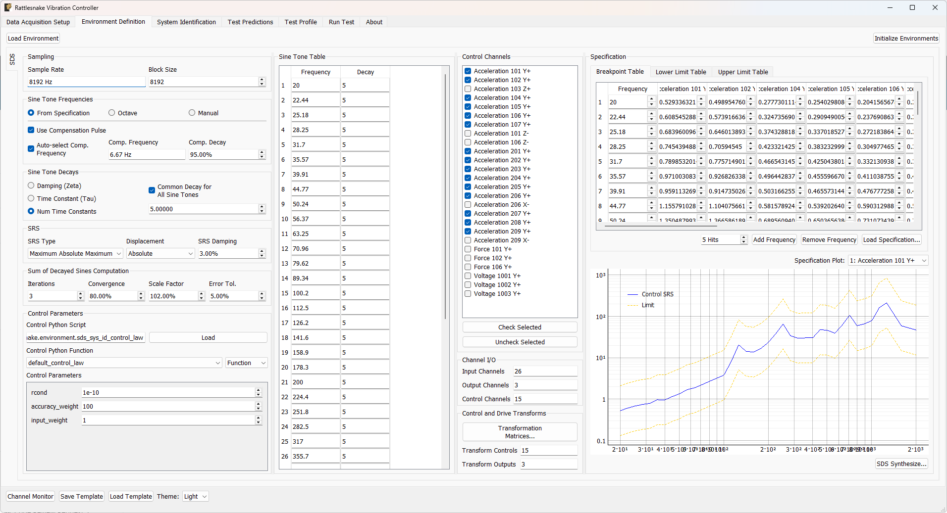
Figure 15.1:UI used to define the MIMO Shock / SDS environment.
15.3.1Sampling Parameters
The Sampling section determines the sample rate and the transient block size used for one SDS hit.
Sample Rate Sample rate in samples per second of the data acquisition hardware, for display only. This is a global parameter and must be set in the Data Acquisition Setup tab.
Block Size The length of the time signal in samples that will be generated. If this is too short for the specified decay, the signals will be truncated.
The block size is important because it defines the duration available for the decayed-sine signal, and the sample rate is important to sufficiently extract the maximum response in the for the SRS computation. Various documentation, such as MIL-STD-810 1, suggest a sample rate of 10x the largest frequency of the shock response spectrum in order to adequately resolve the maximum response.
15.3.2Sine Tone Definition
The SDS environment supports multiple strategies for defining the frequencies used in the decayed-sine table, in the Sine Tone Frequencies portion of the window. This portion also defines if a compensation pulse is used. The compensation pulse is represented internally as an additional decayed-sine row with its own frequency and decay. This is useful in some SDS synthesis workflows to improve the shape or baseline behavior of the transient, often to create a signal with zero net velocity or displacement, so there is not a “snap-back” of the shaker system when the signal ends.
From Specification If selected, the sum of decayed sine signals generated will have a sine tone for each breakpoint in the specified shock response spectra.
Octave If selected, sine tones will be specified using a minimum frequency, maximum frequency, and number of sine tones per octave.
Manual If selected, the user can manually specify sine tone frequencies.
Use Compensation Pulse If selected, a compensation pulse will be utilized. The compensation pulse is often utilized by shock controllers to allow the shaker to return to zero displacement and velocity without a sharp pull-back at the end of the signal. How the compensation pulse is used (if at all) is determined by the control law specified.
Auto-select Compensation Frequency If selected, the frequency of the compensation pulse will be set to 1/3 of the frequency of the lowest sine tone.
Compensation Pulse Frequency Specifies the frequency used by the compensation pulse.
Compensation Decay Specifies the decay parameter used by the compensation pulse. This determines how quickly the compensation pulse decays.
The default option is to specify the Sine Tone Table simply using the frequency breakpoints from the specification SRS as the sine tones in the SDS. In this case, the sine tone table is only for display purposes.
Sine Tone Table The sine tones and decay values used in the test are listed here. If sine tone frequencies or decay values are specified manually, they can be set in this table.
A second option is to specify the the Sine Tone Frequencies by octave. This will involve specifying the minimum and maximum frequency as well as the number of sine tones per octave.
Maximum Frequency This sets the maximum sine tone frequency when specifying sine tones by octave.
Minimum Frequency This sets the minimum sine tone frequency when specifying sine tones by octave.
Tones per Octave This specifies the number of sine tones per octave when sine tones are specified by octave. Each octave is a doubling of the frequency, so sine tones will be logarithmically spaced with the number of tones specified occuring between each doubling of the frequency.
The final approach is to manually specify the Sine Tone Table. In this case, the sine tone table will be editable, and options to add or remove tones will become available.
Sine Tone Table The sine tones and decay values used in the test are listed here. If sine tone frequencies or decay values are specified manually, they can be set in this table.
Add Tone Adds a sine tone to the sine tone table.
Remove Tone Removes the selected sine tone from the table.
15.3.3Decay Definition
The environment supports several equivalent ways to define decay:
damping ( in some literature),
time constant ( in some literature),
number of time constants in the block.
Internally these are converted into the damping-style decay values used during synthesis.
The environment supports either one common decay for all tones, or one decay value per tone.
Decay values are specified in the Sine Tone Decays portion of the window.
Damping (Zeta) If this is selected, decay will be specified as a critical damping ratio (specified by the variable zeta in many formulas).
Time Constant (Tau) If this is selected, decay will be specified as a time constant (specified by the variable tau in many formulas). The time constant is time where the decay has reached 63.2% of the original value.
Number Time Constants If this is selected, decay will be specified as the number of time constants (specified by the variable tau in many formulas within the block. The time constant is time where the decay has reached 63.2% of the original value. The if the number of time constants is set to 5, the decay will be such that the time constant will be 1/5 of the the block size.
Common Decay for All Sine Tones If selected, all sine tones will have the same decay value. If not selected, each sine tone’s decay value can be specified individually.
If a common decay is used, the Sine Tone Decays portion will have the additional widget
Decay Value This is the numerical value used to specify the damping. The meaning of this value will depend on the type of decay selected (Damping, Time Constant, or Num Time Constants).
If decays are specified per sine tone, then they can be entered in the Sine Tone Table portion of the window.
Sine Tone Table The sine tones and decay values used in the test are listed here. If sine tone frequencies or decay values are specified manually, they can be set in this table.
15.3.4SRS Parameters
The SRS section defines how the response SRS is computed. This includes the SRS type, absolute vs. relative displacement convention, and damping. These parameters define both how the specification SRS is computed and how the SRS will be computed from time data.
SRS Type This specifies the type of SRS to compute. There are many different SRS types, including: Primary refers to the peak occuring during the pulse. Residual refers to the peak occuring after the input has ended. Positive, Negative, and Absolute Maximum refer to the maximum positive, maximum negative, and maximum absolute value of response. Primary Positive Largest positive response during input Primary Negative Largest negative response during input Primary Absolute Maximum Largest magnitude response during input Residual Positive Largest positive response after input ends Residual Negative Largest negative response after input ends Residual Absolute Maximum Largest magnitude response after input ends Maximum Positive Largest positive response over entire event Maximum Negative Largest negative response over entire event Maximum Absolute Maximum Largest magnitude response over entire event
Displacement This specifies what displacement type is measured by the SRS. Absolute displacement refers to the oscillator’s motion in inertial space. Relative displacement refers to the oscillator’s motion relative to its base motion.
SRS Damping This is the fraction of critical damping applied to each single degree of freedom oscillator when computing the SRS.
15.3.5SDS Synthesis Parameters
The Sum of Decayed Sines Computation settings control the iterative decayed-sine synthesis algorithm. Because the computation of the SRS is a nonlinear operation on the time response data, an iterative solution is required to compute time response data that fits a given SRS.
Convergence SRS are nonlinear functions, so an optimization routine is required to solve for sum of decayed sine amplitudes that match the SRS. The convergence parameter specifies how much change the optimizer is allowed to make at each step.
Scale Factor The scale factor is applied to the SRS to make the sum of decayed sines match the SRS better, rather than just touching it at the sine tones.
Iterations SRS are nonlinear functions, so an optimization routine is required to solve for sum of decayed sine amplitudes that match the SRS. This value specifies the number of optimization routines to use.
Error Tolerance This is the allowable error in the optimization.
15.3.6Control Law Definition
Like other advanced environments, SDS supports loading a custom Python control law in the Control Parameters section of the window. The definition page allows the user to specify a Python script and function or class within that script to use as a control law. The default control law uses a MIMO inverse-based approach and is described in Section Section 15.8.
Control Python Script Python script used to specify the control law.
Load Opens a file dialog to load in a Python script containing the control law.
Control Python Function Selects the function or class in the Python script to use as the control law.
Control Type Select if the selected control law is a Function, Class, or Interactive Class. This should be detected automatically by inspection; users should not have to adjust this.
Control Parameters Any additional parameters needed by the control law are entered in this area. This area will be automatically populated based on the extra arguments required by the control law.
15.3.7Control Channels
The Control Channels section defines which channels are used to evaluate and control the SRS response. The ordering of these channels determines the ordering of the specification columns when no transformation is used.
Control Channels Channels that are checked will be used as the control channels for this environment. The control channels should be ordered in the specification the same way they are ordered in this list. For example, the first SRS in the specification will correspond to the first checked channel in this list.
Check Selected When clicked, any selected channels in the Control Channels list will be checked, and therefore used as control channels in the environment.
Uncheck Selected When clicked, any selected channels in the Control Channels list will be unchecked, and therefore not used as control channels in the environment.
The Channel I/O section then summarizes the number of physical channels used as inputs, outputs, and control channels.
15.3.8Transformation Matrices
The SDS environment supports both response and excitation transformations, defined in the Control and Drive Transforms section of the window. These work the same way conceptually as in the other environments. A response transformation maps physical control channels into virtual control channels, and an excitation transformation maps physical drive channels into virtual drive signals. See Section 12.8 for the shared transformation-matrix workflow.
Transform Controls A display showing the number of virtual control channels in the environment due to transformation matrices applied to the physical control channels.
Transform Outputs A display showing the number of virtual excitation channels in the environment due to transformation matrices applied to the physical excitation channels.
Transformation Matrices... Open the transformation matrix dialog to allow specification of transformations to virtual control or virtual excitation channels.
15.3.9Test Specification
The SRS specification itself is entered or loaded in the Specification section of the definition page. The user can add or remove breakpoints, edit the required SRS values, edit lower and upper limits, and set the target number of hits. If a user does not wish to control to a specific frequency tone for a specific channel or if upper or lower limits are not desired for that channel and frequency, a Value of NaN can be provided in the loaded specification file, or the value in the table can be set to Disabled.
The specification is added on the Specification section of the window on the Breakpoint Table tab. This is where the breakpoints are added or removed and the control values are modified.
Breakpoint Table This table includes frequency breakpoints and SRS values for the specification.
Add Frequency Adds a frequency breakpoint to the specification table.
Remove Frequency Removes the selected frequency breakpoint from the specification table.
Load Specification Loads specification data from a file.
Number of Hits Specifies the number of hits at full level that should be applied to the test article.
The lower limits are added on the Lower Limit Table tab of the Specification portion of the window.
Lower Limit Table This table specifies lower SRS limits at each breakpoint frequency.
Similarly, upper limits are added on the Upper Limit Table tab of the Specification portion of the window.
Upper Limit Table This table specifies upper SRS limits at each breakpoint frequency.
Finally, there is functionality to display various channels of the specification.
Save Specification Saves specification data to a file.
Specification Channel Specifies which control channel to display on the Specification Plot.
Specification Plot This plot displays the specified SRS for the selected channel.
SDS Synthesize Brings up a dialog box to allow the user to investigate synthesizing ideal data that matches the specified SRS.
15.4System Identification for the MIMO Shock Environment
Like the Random, Sine, and Transient environments, the SDS environment uses a system identification phase defined on the System Identification tab to estimate the transfer functions between the drive channels and control channels. This is shown when all environments are defined and the Initialize Environments button is pressed. The transfer functions are needed because the environment must map desired response behavior back into the corresponding drive signals that can be generated by the control system.
A typical system identification UI for the shock environment is shown in Figure 15.2.
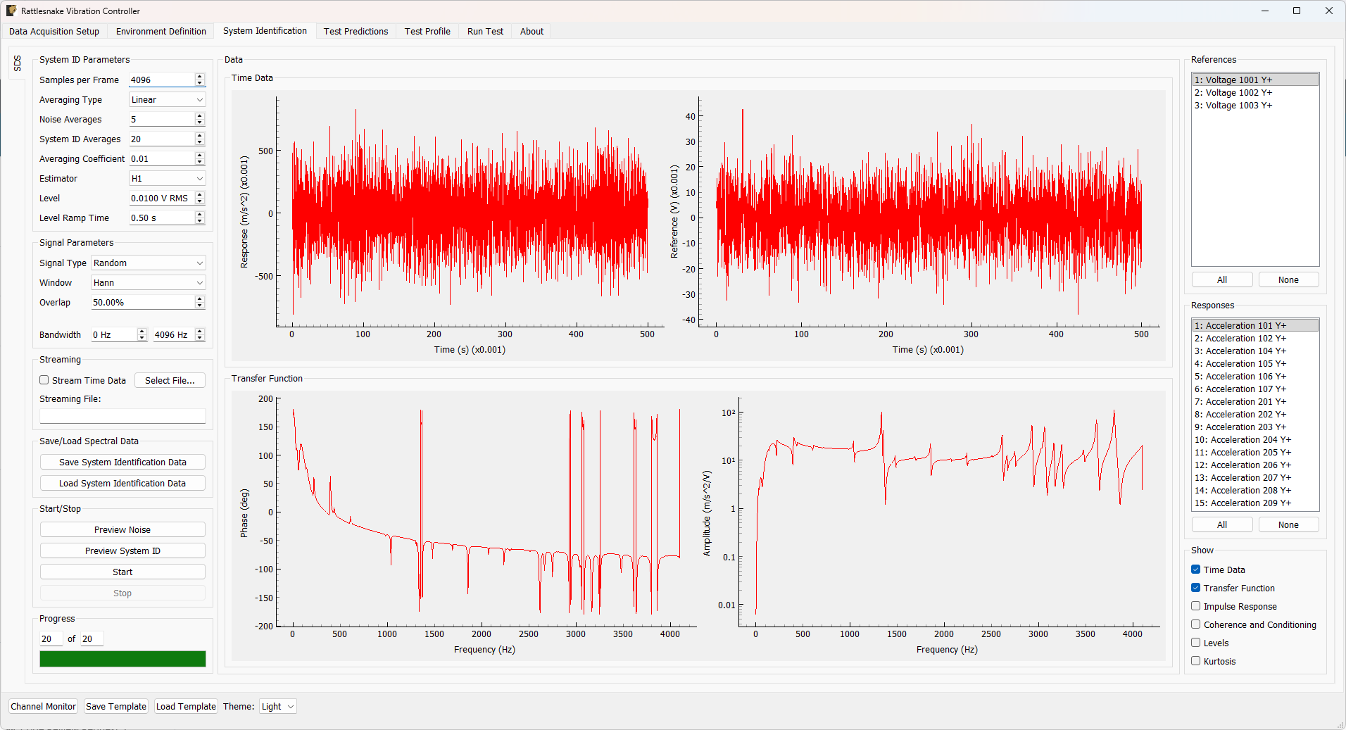
Figure 15.2:System identification UI used by the MIMO Shock / SDS environment.
Rattlesnake’s system identification phase will start with a noise floor check, where the data acquisition records data on all the channels without specifying an output signal. After the noise floor is computed, the system identification phase will play out the specified signals to the excitation devices, and transfer functions will be computed using the responses of the control channels to those excitation signals. Section 3.3 describes the System Identification tab and its various parameters and capabilities.
15.5Test Prediction for the MIMO Shock Environment
Once system identification is complete, the SDS environment can compute a prediction of the drive signals and the resulting response. Note that because the Sum-of-Decays sine calculation is iterative, it can take a bit of time to compute predictions using the default control law, see Section 15.8 for more information on the default control law’s computations.
A representative prediction page is shown in Figure 15.3.
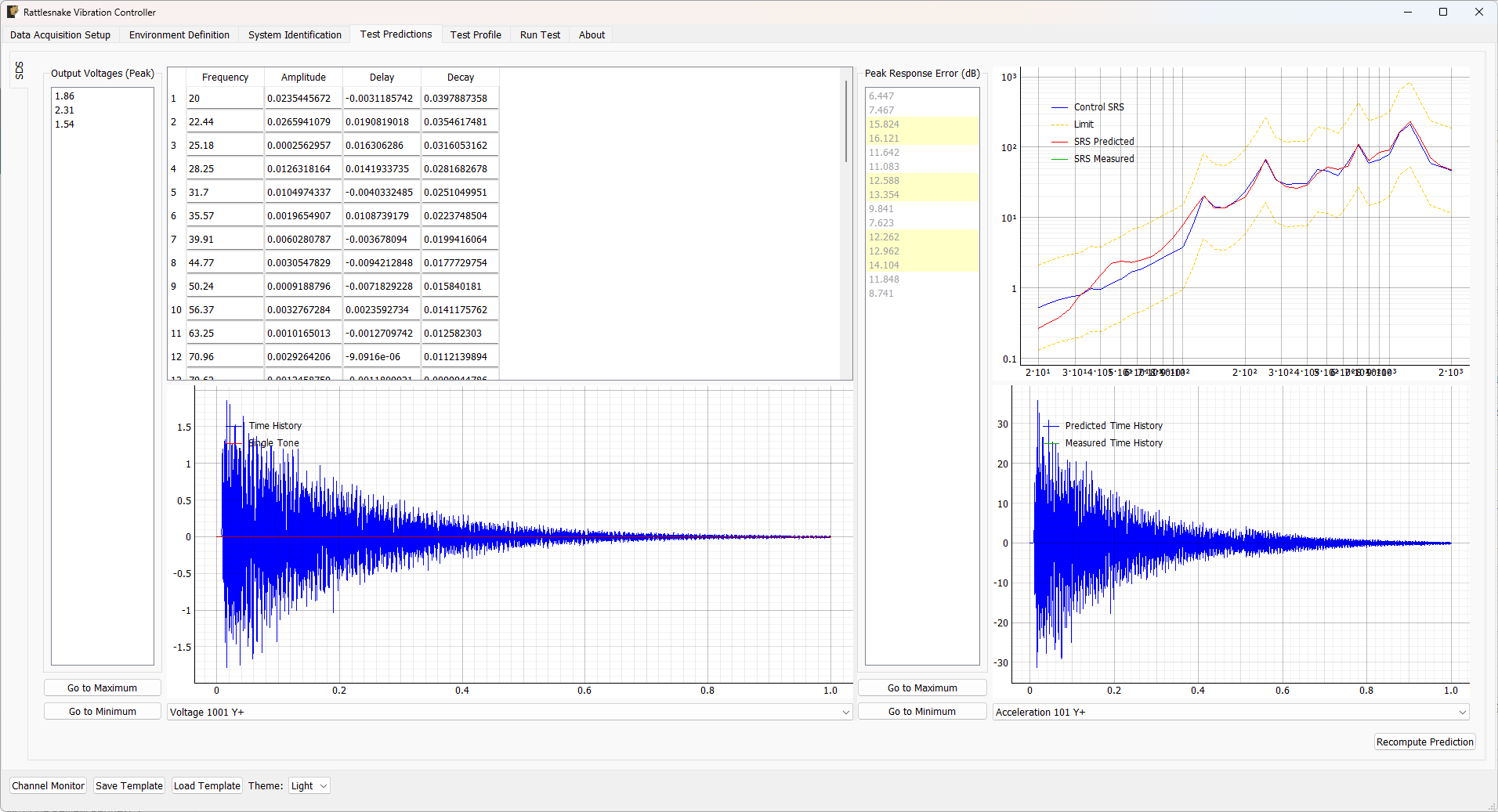
Figure 15.3:Prediction UI used by the MIMO Shock / SDS environment.
The prediction page and associated run-table dialog allow the user to inspect:
the current drive SDS table,
synthesized drive time histories,
predicted response time histories,
predicted response SRS,
peak drive voltages,
peak response errors relative to the SRS specification.
15.5.1Excitation Prediction
The SDS prediction UI is centered around a table of decayed sine terms. For each excitation channel, the table stores:
frequency
amplitude
decay
delay
for each sine tone.
These parameters fully define the synthesized drive transient for that drive channel. The Excitation Display shows the synthesized time history from the tone table. Selecting a row in the tone table will draw that specific sine tone’s contribution to drive transient.
Output Voltages (Peak) Maximum output voltage that will be sent to the shaker to generate the sum-of-decayed-sines signals.
Go to Maximum Voltage Changes the voltage plot to show the excitation signal that reaches the largest maximum value.
Go to Minimum Voltage Changes the voltage plot to show the excitation signal that reaches the smallest maximum value.
Sum of Decayed Sines Table Table showing sum-of-decayed-sines parameters used to generate the output voltage signals.
Excitation Display Displays the time history of the selected voltage signal generated from the sum-of-decayed-sines parameters.
Excitation Selector Specifies the excitation voltage channel to display in the plot.
Recompute Prediction Recomputes the predictions from specified parameters and system identification data.
15.5.2Response Prediction
The right side of the page displays response data. Responses are computed from a convolution of the generated drive signals with the system’s impulse response as measured in the System Identification phase of the controller. These plots allow the user to inspect whether the current open-loop or updated SDS table is likely to meet the specification.
Peak Response Error (dB) Displays the maximum error between the specified SRS and the predicted or measured SRS in decibels.
Go to Maximum Error Changes the response plots to show the control signal that has the largest maximum error.
Go to Minimum Error Changes the response plots to show the control signal that has the smallest maximum error.
Control SRS Plot Displays the SRS for the specification as well as the predicted and measured signals.
Control Time History Plot Displays the time for the predicted and measured response signals.
Response Selector Selects the control channel that will be displayed on the response plots.
15.6Running the MIMO Shock Environment
The Run Test tab of the SDS environment is where actual shock hits are executed and tracked.
A representative run page is shown in Figure 15.4.
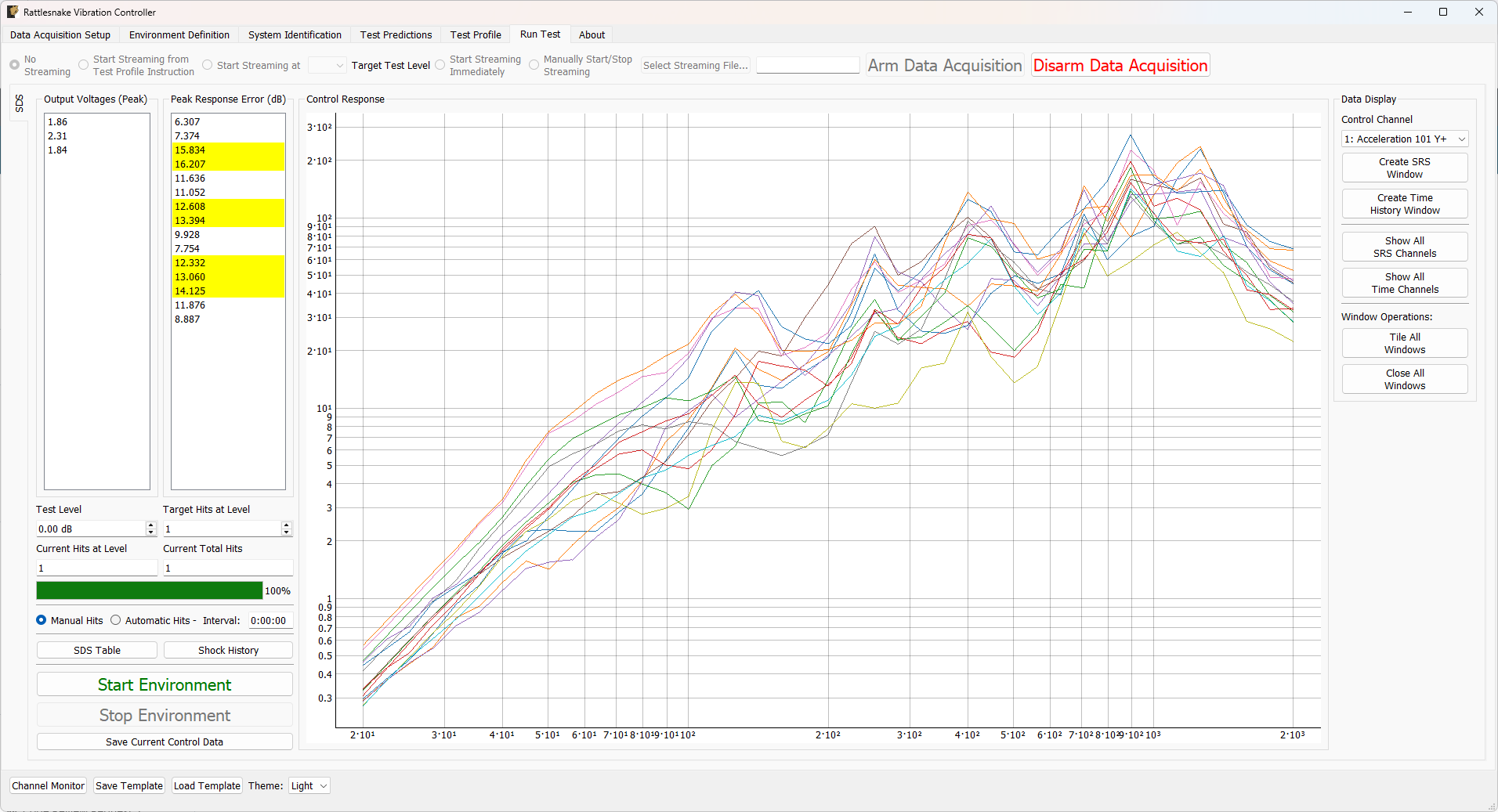
Figure 15.4:Run GUI used by the MIMO Shock / SDS environment.
The SDS run workflow differs from the Random and Sine environments because the natural unit of operation is a single hit, not a continuously running stationary control loop.
The SDS run mode supports:
manual single-hit execution,
automatic repeated hits,
hit counting,
hit history,
manual run-time SDS table drive updates,
optional automatic updates of the SDS table based on the control law,
and post-hit response visualization.
A single SDS hit consists of:
constructing a transient drive waveform from the current SDS table,
playing that transient through the outputs,
measuring the responses,
aligning the measured drive and response to the expected transient,
computing the response SRS,
optionally updating the SDS table through the control law.
This is fundamentally different from the continuously updating loop used by Random Vibration.
The main Run Test tab for the Shock environment contains displays for tracking the overall drive levels and response errors. It also displays the control SRS to give the user a rough idea of the current responses.
Output Voltages (Peak) Displays the peak voltages that will be played to the shaker amplifiers for each drive channel.
Peak Response Error (dB) Displays the maximum error between the specification and the predicted or measured SRS in decibels.
Global Control Response Displays the measured shock response spectra for all control channels.
The tab also has a number of widgets to control the environment as it is running.
Test Level Sets the current test level in dB. 0 dB is the actual test level from the specification. Negative values reduce the shock level; positive values increase it.
Target Hits at Level The number of hits desired at the current test level. If Automatic Hits is used, the measurement will stop after the target number of hits is reached.
Current Hits at Level Displays the current number of hits that have been performed at the current test level.
Current Total Hits Displays the total number of hits performed at any test level.
Progress Bar When automatic impacts are performed, it displays the progress towards the target number of hits at this level.
Manual Hits If selected, the controller will play one shock each time the Start Environment button is pressed.
Automatic Hits If selected, the controller will continue to hit the test article until the Target Hits at Level is reached.
SDS Table Opens up the sum-of-decayed-sines table dialog box, which allows the user to modify the sum-of-decayed-sines parameters manually, make predictions, and view measured data.
Shock History Opens the shock history dialog which shows a history of all shocks applied to the test article.
Start Environment Starts the environment controlling to the specification. Will perform a single hit in manual mode or several hits up to the target hits at level in automatic mode.
Stop Environment Stops the environment prematurely when operating in automatic hit mode.
Save Current Control Data Saves the control data, including specified and measured SRS, to a NumPy, Matlab, or NetCDF4 file.
A brief discussion of the capabilities provided by these widgets is described below.
15.6.1Manual Hits mode
In manual hits mode, each press of Start Environment performs exactly one hit and then returns to idle.
This is useful when dialing in the transient carefully or when the operator wants explicit control over each impact.
15.6.2Automatic Hits mode
In automatic mode, one press of Start Environment begins a sequence of repeated hits separated by the requested interval. The sequence continues until:
the requested number of hits at the selected test level has been reached, or
the operator presses Stop Environment.
If post-hit computations take longer than the requested interval, the next hit is simply launched as soon as the computations finish.
15.6.3Hit counters and history
The SDS run page tracks:
total number of hits,
number of hits at the currently selected test level,
progress toward the requested target hit count,
a full shock history dialog.
Unlike a hardcoded “0 dB only” notion of target-level hits, the SDS environment interprets “hits at level” relative to the currently selected run test level. Thus, if the test level is set to -3 dB, then the displayed hit count and automatic stop logic both operate on the number of historical hits performed at -3 dB.
15.6.4Shock History
Clicking on the Shock History button opens the Shock History dialog shown in Figure 15.5.
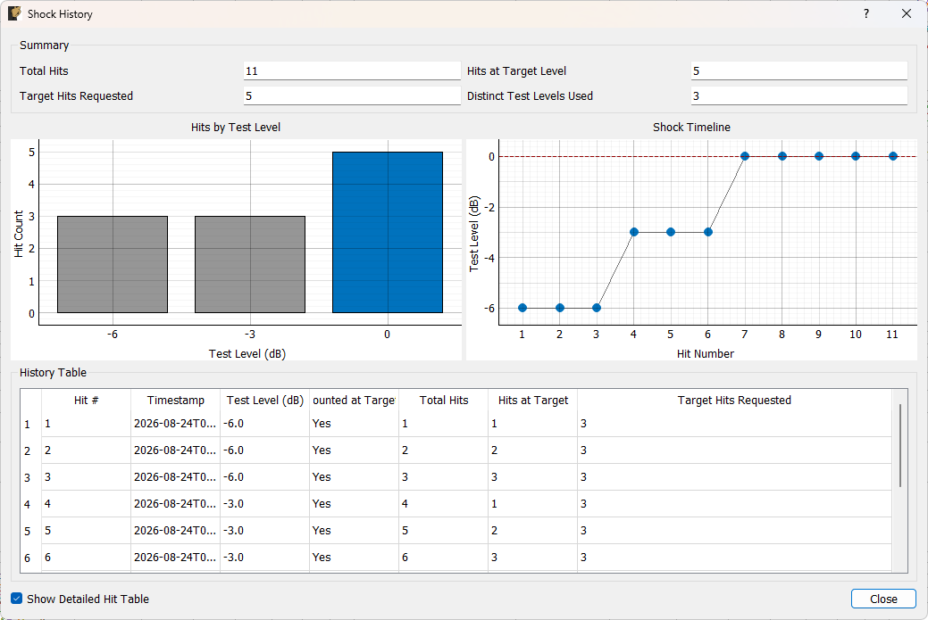
Figure 15.5:Shock History Dialog
The Shock History dialog provides an overview of what has been done to the test article, including:
total hits,
hits at the selected level,
number of distinct test levels used,
a histogram of hits by level,
a chronology plot of hit level versus hit number,
an optional detailed table of every hit.
This is especially useful when many lower-level “dial-in” hits are performed before full-level hits.
There are several numerical displays showing the number of hits.
Total Hits Shows the total number of hits applied to the test article.
Hits at Target Level Displays the total number of hits that were performed at or above the target test level.
Target Hits Requested The total number of hits that were requeted at the target test level by the specification.
Distinct Test Levels Used Displays the total number of different levels used to impact the test article.
There are also graphical displays showing a visual representation of the hit history.
Hit by Test Level Histogram Presents a histogram to display how many hits have been performed at each test level.
Shock Timeline Shows the test level used for each impact.
Close Closes the dialog box.
Show Detailed Hit Table If checked, a detailed hit table containing test level, time stamp, and other information is displayed.
If more detail is desired, a hit table can be shown, showing exactly when each hit occurred.
History Table A detailed hit table containing each impact, its test level, the time stamp, and other information.
15.6.5Run-Time SDS Table
Clicking the SDS Table button will bring up a dialog containing a real-time display of the SDS table that is used to generate voltage signals. This is shown in Figure 15.6.
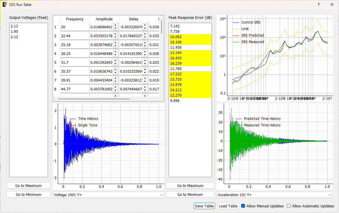
Figure 15.6:Shock History Dialog
Depending on which options are checked the user can manually or the control law can automatically update the values in this table. When values are updated, the control law will automatically make response predictions based on the new drive signals. When measurements are obtained, the measured data will also be plotted on the response sections. This allows users or the control law to tune the controller as the run is progressing.
This dialog is particularly important because the SDS environment is table-driven: the current SDS table defines the transient that will be played on the next hit.
The left side of the window focuses on the drive signals:
Output Voltages (Peak) Maximum output voltage that will be sent to the shaker to generate the sum-of-decayed-sines signals.
Go to Maximum Voltage Changes the voltage plot to show the excitation signal that reaches the largest maximum value.
Go to Minimum Voltage Changes the voltage plot to show the excitation signal that reaches the smallest maximum value.
Sum of Decayed Sines Table Table showing sum-of-decayed-sines parameters used to generate the output voltage signals.
Excitation Display Displays the time history of the selected voltage signal generated from the sum-of-decayed-sines parameters.
Excitation Selector Specifies the excitation voltage channel to display in the plot.
The right side of the window focuses on measured responses and responses predicted from the updated drive voltages based on transfer functions.
Peak Response Error (dB) Displays the maximum error between the specified SRS and the predicted or measured SRS in decibels.
Go to Maximum Error Changes the response plots to show the control signal that has the largest maximum error.
Go to Minimum Error Changes the response plots to show the control signal that has the smallest maximum error.
Control SRS Plot Displays the SRS for the specification as well as the predicted and measured signals.
Control Time History Plot Displays the time for the predicted and measured response signals.
Response Selector Selects the control channel that will be displayed on the response plots.
Save Table Saves the current sum-of-decayed-sines table to a NumPy, CSV, or Excel file.
Load Table Loads a sum-of-decayed-sines table from a NumPy, CSV, or Excel file.
Allow Manual Updates If selected, the user can manually update the sum-of-decayed-sines parameters by modifying values in the table. If not selected, the user cannot change these parameters.
Allow Automatic Updates If selected, the control law will be run after each impact to potentially update the sum-of-decayed-sines parameters automatically.
15.6.6Displaying Data
In addition to the main UI showing all of the control SRSs and the Run Table showing predictions and measured responses, SRS and time histories from individual channels can be shown in separate windows using the operations in the Data Display. Representative windows are shown in Figure 15.7 and Figure 15.8.
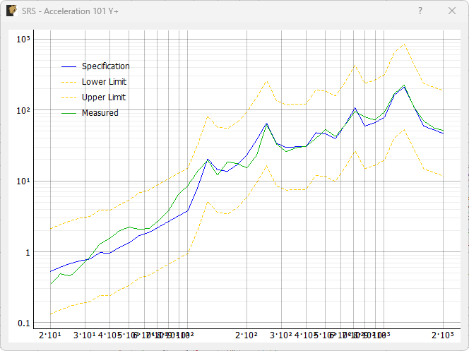
Figure 15.7:Control SRS Window
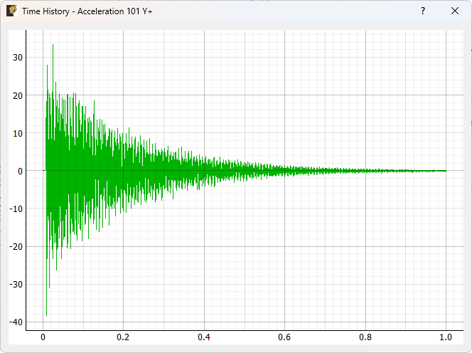
Figure 15.8:Control Time Window
Control Channel Selector Specifies the channel for which a SRS or Time History plot will be created.
Create SRS Window Creates a window displaying the specified and measured SRS for the selected channel.
Create Time History Window Creates a window displaying the measured time history for the selected channel.
Show All SRS Channels Creates an SRS window for each control channel in the test and then tiles the windows across the main monitor.
Show All Time Channels Creates a window showing the time response for all control channels and tiles them across the main monitor.
Tile All Windows Tiles all existing windows over the main monitor
Close All Windows Close all existing SRS or Time History windows.
15.7Output NetCDF File Structure
Like the other environments in Rattlesnake, the SDS environment stores its metadata in a netCDF group whose name matches the environment name.
Because the SDS environment derives from the shared system-identification infrastructure, its netCDF group contains SDS-specific metadata, shared system-ID metadata, and, when saving control data, the current SDS table, most recent hit data, and hit history.
Due to the complexity of the metadata for the SDS environment, the metadata is spread between the main group and several subgroups, each handling a specific portion of the metadata.
15.7.1NetCDF Dimensions
The SDS environment creates the following dimensions in its netCDF group.
control_channels — the number of physical control channels.
specification_channels — the number of specification/control channels after transformation.
tone_data_size — the number of tone-definition values used when tones are specified explicitly.
num_decays — the number of explicitly stored decay values if decays are not common across tones.
num_frequencies — the number of SRS frequency lines in the specification.
num_spec_signals — the number of control/specification channels in the SRS specification.
sds_frequencies — the number of frequencies in the run SDS table when saving control data.
sds_drive_channels — the number of drive channels in the run SDS table when saving control data.
hit_history_length — the number of historical hits when saving control data.
response_transformation_rows — the number of rows in the response transformation matrix, if one is defined.
response_transformation_cols — the number of columns in the response transformation matrix, if one is defined.
reference_transformation_rows — the number of rows in the excitation/output transformation matrix, if one is defined.
reference_transformation_cols — the number of columns in the excitation/output transformation matrix, if one is defined.
15.7.2NetCDF Attributes
The SDS environment group stores both shared system-ID attributes and SDS-specific attributes on the environment’s netCDF group.
sysid_sample_rate — the sample rate used during system identification.
sysid_frame_size — the number of samples per frame used during system identification.
sysid_averaging_type — the averaging scheme used in the system identification (
LinearorExponential).sysid_noise_averages — the number of frames used in the noise-floor characterization.
sysid_averages — the number of frames used in the transfer-function measurement.
sysid_exponential_averaging_coefficient — the exponential averaging coefficient when exponential averaging is selected.
sysid_estimator — the estimator used for FRF computation, such as H1, H2, H3, or Hv.
sysid_level — the excitation level used during system identification.
sysid_level_ramp_time — the ramp time used to transition into and out of the system identification level.
sysid_signal_type — the signal type used during system identification.
sysid_window — the window applied to the time frames during system identification.
sysid_overlap — the overlap fraction used during system identification.
sysid_burst_on — the fraction of the burst-random frame that is “on,” if burst random is used.
sysid_pretrigger — the fraction of the frame used as pretrigger for burst-random system identification.
sysid_burst_ramp_fraction — the fraction of the burst-random “on” interval used to ramp the burst up and down.
sysid_low_frequency_cutoff — the low-frequency cutoff used during system identification.
sysid_high_frequency_cutoff — the high-frequency cutoff used during system identification.
block_size — the number of samples in one SDS hit block.
When saving current control data after or during a run, additional scalar attributes are also stored, including:
current_test_level_db — the run test level in dB,
current_test_level_scale — the corresponding linear scale factor,
total_hits — cumulative number of hits,
hits_at_target — cumulative number of hits at the currently selected test level,
allow_automatic_updates — whether the run table is being automatically updated.
15.7.3NetCDF Variables
Only one variable consistently exists in the root environment group.
control_channel_indices — the indices of the physical control channels in the environment. These indices correspond to the physical channels that define the control degrees of freedom before any response transformation is applied. Type: 32-bit integer; Dimensions:
control_channels
If transformation matrices are defined, the following variables may also be present directly on the environment group:
response_transformation_matrix — the transformation matrix applied to the physical control channels. Type: 64-bit float; Dimensions:
specification_channels×control_channelsreference_transformation_matrix — the transformation matrix applied to the physical drive channels. Type: 64-bit float; Dimensions:
reference_transformation_rows×reference_transformation_cols
These variables are omitted when no transformation is used.
15.7.4Tone Parameters Subgroup
The subgroup tone_parameters stores:
tone_data_size (dimension) — This dimension will only exist if the
tone_datavariable exists. It will be3if the tone strategy is “octave spacing”; otherwise, it will be the number of manual tones specified.strategy (attribute) — A numerical value representing the tone-generation strategy:
from specification (
strategy == 0)octave spacing (
strategy == 1)manual tones (
stragegy == 2)
tone_data (variable, optional) — the associated tone-definition values. If the tone strategy is “from specification”, this variable will not exist. If the tone strategy is “octave spacing”, it will have three values, which are the minimum frequency, maximum frequency, and tones per octave. If the tone strategy is “manual tones”, it will include each frequency. Type: 64-bit float; Dimensions:
tone_data_size.
15.7.5Compensation Pulse Subgroup
The subgroup compensation_pulse_parameters stores the following attributes:
use_compensation_pulse — whether a compensation pulse is enabled. It is represented as a boolean integer with
0representing no compensation pulse used and1when using a compensation pulse.compensation_frequency — compensation frequency if specified explicitly. If this value is not defined and
use_compensation_pulse == 1, then the frequency is automatically selected.compensation_decay — compensation decay value. This value is only defined if a compensation pulse is used.
15.7.6Decay Parameters Subgroup
The subgroup decay_parameters stores the following attributes:
decay_strategy — an integer describing how the decay values were originally specified. The supported values correspond to the
DecayStrategyenumeration:0= damping1= time constant2= number of time constants
common_decay — a boolean integer indicating whether a single common decay value is used for all tones. A value of
1means a single decay value is used for all tones, while0means one decay value is specified per tone.
This subgroup also stores one of the following:
decay_data — if
common_decay == 1, thendecay_datais stored as a scalar attribute representing the common decay value.num_decays (dimension) and decay_data (variable) — if
common_decay == 0, then a dimensionnum_decaysis created and the decay values are stored as a one-dimensional variable. Type: 64-bit float; Dimensions:num_decays.
15.7.7SRS Parameters Subgroup
The subgroup srs_parameters stores the following attributes:
srs_type — an integer identifying the SRS response type, corresponding to the
SRSTypeenumeration.Primary Positive = 1
Primary Negative = 2
Primary Absolute Maximum = 3
Residual Positive = 4
Residual Negative = 5
Residual Absolute Maximum = 6
Maximum Positive = 7
Maximum Negative = 8
Maximum Absolute Maximum = 9
srs_displacement — an integer identifying whether absolute (
1) or relative displacement (-1) is used in the SRS computation.srs_damping — the damping ratio used in the SRS computation.
These values fully define how the environment computes SRS values from transient response data.
15.7.8SDS Synthesis Parameters Subgroup
The subgroup sds_parameters stores the following attributes:
iterations — the number of iterations used by the SDS synthesis algorithm.
convergence — the convergence factor used by the iterative SDS synthesis.
scale_factor — a multiplicative factor applied during SDS synthesis to bias the result toward slightly over-hitting the target.
error_tolerance — the allowable fractional error used during SDS synthesis.
These values define how the response-side sum-of-decayed-sines synthesis is performed before the MIMO inverse is solved.
15.7.9Specification Parameters Subgroup
The subgroup specification_parameters stores the user’s SRS specification. It contains the following attribute:
num_hits — the requested number of hits to perform at the selected level.
The subgroup also stores the following dimensions:
num_frequencies — the number of frequency lines in the specification.
num_spec_signals — the number of control/specification channels.
The following variables are then defined:
frequencies — the specification SRS frequencies in Hz. Type: 64-bit float; Dimensions:
num_frequenciessrs_spec — the required SRS amplitudes at each specification frequency for each control channel. Type: 64-bit float; Dimensions:
num_frequencies×num_spec_signalssrs_lower_limit — the lower SRS limits at each specification frequency for each control channel. Type: 64-bit float; Dimensions:
num_frequencies×num_spec_signalssrs_upper_limit — the upper SRS limits at each specification frequency for each control channel. Type: 64-bit float; Dimensions:
num_frequencies×num_spec_signals
If control or limits are not required for particular frequency/channel combinations, those entries may be NaN.
15.7.10Control Parameters Subgroup
The subgroup control_parameters stores metadata describing the SDS control law. It contains the following attributes:
control_type — an integer specifying how the control law is implemented. The values correspond to the
ControlLawTypeenumeration:0= function1= class2= interactive class
control_script — the Python module or script path containing the control law.
control_object — the function or class name inside the control script.
A nested subgroup named control_extra_parameters is also created. This subgroup stores each additional control-law parameter as an attribute on the subgroup, using the parameter name as the attribute key.
This allows arbitrary scalar control-law settings to be stored without changing the netCDF schema.
15.7.11Saved Control Data
When the user saves current SDS control data from the Run Test page rather than streaming, the netCDF file additionally stores the current run state, including:
the current SDS table:
run_table_frequency
run_table_amplitude
run_table_delay
run_table_decay
the most recent measured drive time history:
measured_drive_time_history
the most recent measured response time history:
measured_response_time_history
the most recent measured response SRS:
measured_response_srs
convenience copies of the specification arrays:
specification_frequencies_array
specification_srs
specification_lower_limit
specification_upper_limit
hit history arrays:
hit_index
timestamp
test_level_db
counted_at_target
total_hits
hits_at_target
target_hits_at_level
These are in addition to the environment metadata already described above.
If a run SDS table is stored, the following dimensions are created:
sds_frequencies — the number of rows in the current SDS table.
sds_drive_channels — the number of drive channels represented in the SDS table.
The following variables are then stored:
run_table_frequency — the frequencies of the current SDS table. Type: 64-bit float; Dimensions:
sds_frequenciesrun_table_amplitude — the amplitudes of the current SDS table. Type: 64-bit float; Dimensions:
sds_frequencies×sds_drive_channelsrun_table_delay — the delays of the current SDS table. Type: 64-bit float; Dimensions:
sds_frequencies×sds_drive_channelsrun_table_decay — the decays of the current SDS table. Type: 64-bit float; Dimensions:
sds_frequencies×sds_drive_channels
If the most recent measured drive signal is available, the following dimensions are created:
measured_drive_channels
measured_drive_samples
and the variable
measured_drive_time_history — the measured drive signal from the most recent hit. Type: 64-bit float; Dimensions:
measured_drive_channels×measured_drive_samples
If the most recent measured control response is available, the following dimensions are created:
measured_response_channels
measured_response_samples
and the variable
measured_response_time_history — the measured response signal from the most recent hit. Type: 64-bit float; Dimensions:
measured_response_channels×measured_response_samples
If the most recent measured response SRS is available, the following dimensions are created:
measured_srs_frequencies
measured_srs_channels
and the variable
measured_response_srs — the measured response SRS from the most recent hit. Type: 64-bit float; Dimensions:
measured_srs_frequencies×measured_srs_channels
To make post-run analysis easier, the current specification is also written explicitly to the saved control-data file even though it is already represented in the metadata subgroup. The following dimensions are created:
specification_frequencies
specification_channels
The following variables are stored:
specification_frequencies_array — the specification SRS frequency vector. Type: 64-bit float; Dimensions:
specification_frequenciesspecification_srs — the specified SRS values. Type: 64-bit float; Dimensions:
specification_frequencies×specification_channelsspecification_lower_limit — the lower SRS limits. Type: 64-bit float; Dimensions:
specification_frequencies×specification_channelsspecification_upper_limit — the upper SRS limits. Type: 64-bit float; Dimensions:
specification_frequencies×specification_channels
When saving current SDS control data, the following scalar run-state attributes are written:
current_test_level_db — the currently selected SDS run level in dB.
current_test_level_scale — the corresponding linear scale factor.
total_hits — the cumulative number of hits performed in the environment.
hits_at_target — the cumulative number of hits at the currently selected test level.
allow_automatic_updates — 1 if automatic SDS table updates are enabled, 0 otherwise.
The hit history is stored in a flattened array form for easy analysis. The dimension
hit_history_length — the number of entries in the hit history
is created, and then the following arrays are stored:
hit_index — integer index of each hit. Type: integer; Dimensions:
hit_history_lengthtimestamp — timestamp string for each hit. Type: string; Dimensions:
hit_history_lengthtest_level_db — test level in dB at which the hit was performed. Type: 64-bit float; Dimensions:
hit_history_lengthcounted_at_target — boolean/int flag indicating whether the hit counted toward the currently selected target-level count. Type: integer/bool; Dimensions:
hit_history_lengthtotal_hits — cumulative total hit count after that hit. Type: integer; Dimensions:
hit_history_lengthhits_at_target — cumulative hit count at the selected level after that hit. Type: integer; Dimensions:
hit_history_lengthtarget_hits_at_level — requested target number of hits at that level at the time of the run. Type: integer; Dimensions:
hit_history_length
This structure allows a saved SDS run file to serve not only as a metadata archive, but also as a record of what was actually done to the test article over the course of the run.
15.8Writing a Custom SDS Control Law
The SDS environment supports custom control laws through a Python function or class, and the current default implementation is a useful reference because it demonstrates the full chain from:
specification SRS,
to response target construction,
to MIMO inversion,
to drive amplitudes, phases, and delays.
A custom SDS control law is expected to produce updated SDS table quantities:
amplitudes,
decays,
delays
for each decayed-sine term and drive channel.
15.8.1What the default SDS control law does
The current default control law, implemented in sds_sys_id_control_law.py, proceeds in several stages.
15.8.1.1Stage 1: Build the target response SRS
The control law begins from the target SRS stored in the environment metadata. This target is defined for each control channel at the SDS frequencies.
15.8.1.2Stage 2: Generate a decayed-sine representation of the target response
For each control channel, helper routines synthesize a decayed-sine signal whose resulting SRS approximates the target SRS. This produces:
sine frequencies,
provisional response amplitudes,
decays,
delays.
15.8.1.3Stage 3: Interpolate the FRF matrix
The measured system-identification FRFs are interpolated onto the SDS frequencies.
15.8.1.4Stage 4: Solve a MIMO inverse with optimized response phases
At each SDS frequency, the control law solves a MIMO inverse problem using the transfer function matrix and an optimized set of response phases. This produces a complex drive vector for that frequency.
This is done using a pseudoinverse-based solve with phase-target optimization to balance:
response accuracy,
and drive effort.
15.8.1.5Stage 5: Convert complex drives into amplitudes and delays
The complex drive values are converted into:
drive amplitudes,
drive phases,
and the phases are converted to delays via
15.8.1.6Stage 6: Optionally include a compensation pulse row
If a compensation pulse is enabled, the returned SDS table includes an additional row for it. The current default control law does not yet try to optimize the compensation pulse itself, so the compensation row is currently appended with zero amplitude.
15.8.2Function-Based SDS Control Laws
The simplest way to implement a custom SDS control law is as a Python function.
This is the same style used by the current default control law.
A function-based control law is best when the control calculation is mostly stateless, all required information is naturally available from the current call, or the user wants the simplest possible implementation.
A function-based SDS control law must accept the core arguments expected by the environment and must return
amplitudes
decays
delays for each sine tone.
15.8.2.1Expected function signature
A function-based SDS control law should have a signature compatible with:
def my_sds_control_law(
    environment_metadata,
    sysid_data,
    last_response_srs=None,
    last_response_signals=None,
    last_drive_amplitudes=None,
    last_drive_decays=None,
    last_drive_delays=None,
    last_drive_signals=None,
    **kwargs,
):
    ...
    return amplitudes, decays, delays
The exact parameter order and keyword argument names need not match exactly, but the function must be callable using keyword arguments corresponding to the environment’s expected call pattern.
The function arguments are:
environment_metadata — the full SDS environment metadata object, including specification, tone strategy, decay strategy, SRS parameters, and control-law configuration.
sysid_data — the system identification package, including the FRFs and related system-ID outputs.
last_response_srs — the most recent measured response SRS from a completed hit, scaled back to full test level.
last_response_signals — the most recent measured response time histories from a completed hit, scaled back to full test level.
last_drive_amplitudes — the amplitudes from the previous SDS table used for the last hit.
last_drive_decays — the decays from the previous SDS table used for the last hit.
last_drive_delays — the delays from the previous SDS table used for the last hit.
last_drive_signals — the most recent measured drive time histories, scaled back to full test level.
These last-* quantities may be None during the initial prediction stage, before any actual hit has been performed.
Additional keyword arguments can be specified in the function signature, but they must have type hints assigned to allow the UI to populate the correct interface to capture that argument. See Section 15.8.5 for more information.
15.8.2.2Return values
The function must return three arrays:
amplitudes
decays
delays
These are expected to be shaped consistently with the environment’s SDS table:
one row per SDS frequency, including the compensation-pulse row if enabled,
one column per drive channel.
Thus, if there are SDS frequencies and drive channels, the returned arrays should each have shape
If the compensation pulse is enabled, the final row corresponds to that compensation term.
15.8.2.3Minimal example
A minimal function-based control law might look like:
def my_sds_control_law(
    environment_metadata,
    sysid_data,
    last_response_srs=None,
    last_response_signals=None,
    last_drive_amplitudes=None,
    last_drive_decays=None,
    last_drive_delays=None,
    last_drive_signals=None,
    **kwargs,
):
    frequencies = environment_metadata.get_sds_frequencies_w_compensation_pulse()
    num_drive_channels = environment_metadata.num_reference_channels

    amplitudes = np.zeros((frequencies.size, num_drive_channels))
    decays = np.tile(
        environment_metadata.get_sds_decays_w_compensation_pulse()[:, np.newaxis],
        (1, num_drive_channels),
    )
    delays = np.zeros((frequencies.size, num_drive_channels))

    return amplitudes, decays, delays
This example is not useful as a real controller as it only outputs zeros, but it shows the required structure.
15.8.3Class-Based SDS Control Laws
A class-based control law is appropriate when the user wants to preserve state between calls.
This is useful when the control law needs to remember things like:
optimization history,
phase-target history,
trust-region or step-size information,
previous successful SDS tables,
hit-dependent weighting or adaptation logic.
A class makes it easy to keep persistent internal state without rederiving or reparsing everything on every control-law call.
This is especially valuable for SDS because the environment is naturally hit-based and iterative.
15.8.3.1Expected class structure
A class-based SDS control law in the SDS environment is expected to provide at least:
a constructor
__init__(...)a
system_id_update(...)methoda
control(...)method
A typical structure might look like:
class MySDSControlLaw:
    def __init__(
        self,
        environment_metadata,
        sysid_data,
        last_response_srs=None,
        last_drive_amplitudes=None,
        last_drive_decays=None,
        last_drive_delays=None,
        **kwargs,
    ):
        self.environment_metadata = environment_metadata
        self.sysid_data = sysid_data
        self.extra_parameters = kwargs

    def system_id_update(self, sysid_data):
        self.sysid_data = sysid_data

    def control(
        self,
        last_response_srs,
        last_response_signals,
        last_drive_amplitudes,
        last_drive_decays,
        last_drive_delays,
        last_drive_signals,
    ):
        ...
        return amplitudes, decays, delays
In practice, the current example class-based implementation (DefaultSDSControlLaw) uses the following pattern:
__init__(...)stores the environment metadata, the system identification package, and any extra user-provided parameters,system_id_update(...)performs the main SDS-table computation using the specification and FRFs,control(...)returns the most recently computed amplitudes, decays, and delays.
This means that a class-based SDS control law does not have to recompute the entire SDS table on every control(...) call. A valid implementation may instead compute the table once in system_id_update(...), cache it internally, and then either:
return it unchanged, or
apply incremental updates based on the most recent measured hit data.
15.8.3.2Lifecycle of a class-based control law
A class-based SDS control law participates in the environment lifecycle as follows.
15.8.3.2.1__init__(...)
The environment constructs the class during environment initialization and passes in:
environment metadata,
current system-ID package,
initial response/drive data if available,
and any extra control-law parameters.
This is the correct place to:
store persistent metadata,
parse user parameters,
initialize caches,
and prepare internal data structures.
15.8.3.2.2system_id_update(...)
When the system identification changes or is reloaded, this method is called so the control law can update any FRF-dependent internal state.
This is useful if the class wants to store:
interpolated FRFs,
pseudoinverse matrices,
or any derived transfer-function quantities.
15.8.3.3control(...)
This method is called to obtain the SDS table that should be used for prediction or for the next hit.
A class-based control law may choose to:
recompute the SDS table from scratch,
apply a hit-to-hit update to a previously computed table,
or simply return the most recently cached table.
The current example class-based control law uses the third approach: it performs the main inversion and table construction in system_id_update(...), then control(...) returns the most recently computed:
amplitudes,
decays,
delays.
This is a valid pattern when the control law is effectively open-loop after the most recent system-identification update.
15.8.3.4Practical guidance
A class-based SDS control law should still preserve the same core responsibilities as the function-based version:
use the SRS specification as the response target,
use the system identification data to relate response to drive,
produce an SDS table that can be synthesized by the environment,
optionally adapt that table based on previous measured hits.
The difference is that a class can preserve internal state between those calls.
15.8.4Interactive SDS Control Laws
The SDS environment also supports an interactive class mode, intended for more advanced workflows where the control law may need to exchange parameters or commands with a UI object.
This is the most advanced and most stateful control-law style.
An interactive control law may be appropriate when the user wants:
custom runtime parameter tuning,
custom visualization,
or a dialog/window dedicated to the control algorithm itself.
In this mode, the environment can:
update the control-law parameters dynamically,
send interactive commands,
and allow the control law to return information back to the UI.
This mode is best suited to research-oriented or experimental control implementations.
15.8.5Additional Control-Law Parameters and GUI Population
One of the most useful SDS features is that additional control-law parameters can be exposed automatically in the Environment Definition page when a Python control function is loaded.
When the user loads a Python module containing candidate SDS control laws, the UI inspects the available functions and classes and identifies which ones are valid control laws.
A function is considered valid if it contains the required arguments:
environment_metadatasysid_datalast_response_srslast_response_signalslast_drive_amplitudeslast_drive_decayslast_drive_delayslast_drive_signals
Any additional keyword-capable arguments beyond these required arguments are treated as extra control parameters.
The UI can automatically create widgets for extra parameters when the parameter type annotation is one of:
intfloatstran
Enumsubclass
If the parameter has a supported type annotation, the UI creates a matching widget automatically:
int→ integer spin boxfloat→ scientific double spin boxstr→ text editEnum→ combo box
If the parameter has an unsupported annotation but provides a default value, the function can still be loaded, but that argument is not exposed as an editable widget.
For example, a function like:
def my_sds_control_law(
    environment_metadata,
    sysid_data,
    last_response_srs=None,
    last_response_signals=None,
    last_drive_amplitudes=None,
    last_drive_decays=None,
    last_drive_delays=None,
    last_drive_signals=None,
    *,
    rcond: float = 1e-10,
    accuracy_weight: float = 100.0,
    input_weight: float = 1.0,
):
    ...
will automatically expose widgets for:
rcondaccuracy_weightinput_weight
in the SDS Environment Definition page.
The UI collects those values into a dictionary and stores them in the ControlParameters metadata object.
For class-based SDS control laws, the same idea applies to the constructor. The UI inspects the __init__(...) signature of the class and exposes any supported additional keyword-capable constructor arguments as editable GUI parameters, while ignoring the standard runtime-provided SDS arguments such as the environment metadata and system identification package.
When the environment later calls the function-based control law or class control law’s __init__(...) method, those parameters are unpacked as keyword arguments:
control_law(
    environment_metadata=...,
    sysid_data=...,
    last_response_srs=...,
    last_response_signals=...,
    last_drive_amplitudes=...,
    last_drive_decays=...,
    last_drive_delays=...,
    last_drive_signals=...,
    **control_parameters,
)
Thus, extra control-law arguments are simply normal Python keyword arguments whose values are supplied by the UI.
If you want your control law to expose user-tunable parameters in the GUI, the easiest way is to:
include the standard required SDS arguments,
add additional keyword arguments,
annotate them with supported Python types,
provide reasonable default values.
That way the SDS UI can automatically build the needed widgets.
15.8.6What a Custom SDS Control Law Must Do
A replacement SDS control law should preserve the same broad responsibilities, even if the mathematics differ.
At minimum, a custom implementation should be able to:
accept and store specification information,
accept updated system identification results,
compute an initial or updated SDS table,
optionally preserve state between hits,
return amplitudes, decays, and delays in the expected SDS table format.
In other words, even if a custom SDS control law uses a completely different synthesis or inversion strategy, it still needs to fit into the same environment lifecycle and data contract.
15.8.7Practical Guidance for Implementing a Replacement
15.8.7.1Preserve state explicitly if needed
If your control law needs to remember things like:
previous optimization seeds,
previous phase targets,
previous fitted errors,
or any iterative tuning history,
then use a class-based implementation rather than trying to reconstruct that state each call.
15.8.7.2Be careful about coordinate systems
The control law may be operating on:
physical control channels,
transformed response coordinates,
physical drive channels,
transformed drive coordinates.
A custom implementation should ensure that:
the specification,
the transfer functions,
and the returned SDS table
are all interpreted in mutually consistent coordinates.
15.8.7.3Respect the expected return format
The SDS environment expects arrays shaped like the current SDS table. In particular:
one row per SDS frequency,
one column per drive channel,
compensation-pulse row included if the environment expects it.
Returning the wrong shape will generally cause the environment to fail or produce invalid synthesis.
15.8.7.4Remember that measured data are scaled back to full level
During run-time postprocessing, the SDS environment scales measured response and drive data back up to the nominal full level before passing them to the control law. A custom control law therefore receives normalized data appropriate for direct comparison to the specification.
15.8.7.5Think carefully about hit-based iteration
Unlike Random or Sine, the SDS environment evolves one hit at a time. A replacement control law should therefore think in terms of:
what to do before the first hit,
what to do after a completed hit,
whether to preserve state between hits,
and whether automatic updates are intended to occur at all.
If automatic SDS table updates are disabled, the environment may skip calling the control law entirely after hits, so a custom implementation should be designed with that workflow in mind.
15.8.8Summary
A custom SDS control law in Rattlesnake may be implemented as either:
a Python function,
a stateful Python class,
or an interactive class.
The current default implementation is function-based, but class-based implementations are often a natural fit for SDS because the problem is iterative and hit-based.
The key requirement is that the control law must participate correctly in the SDS environment lifecycle and return:
amplitudes,
decays,
delays
in a form that the environment can synthesize and execute.
- United States Department of Defense. (2019). MIL-STD-810H: Environmental Engineering Considerations and Laboratory Tests (Standard MIL-STD-810H). U.S. Army Test. https://quicksearch.dla.mil/qsDocDetails.aspx?ident_number=35978