14Multiple Input/Multiple Output Sine Control
The MIMO Sine environment in Rattlesnake is used to generate deterministic sinusoidal excitations at one or more drive channels so that the measured response at one or more control channels matches a prescribed specification. Unlike the Random Vibration environment, which operates on power spectral density matrices, the Sine environment operates on explicitly defined amplitude, phase, frequency, and sweep-rate information over time.
At a high level, the MIMO Sine environment does three things:
defines one or more sine sweeps as a specification,
uses a system identification phase to estimate the transfer functions between drive and response channels,
computes drive signals that should reproduce the specified response amplitudes and phases, and then updates those drives during a run based on measured tracking data.
The environment supports:
multiple control channels,
multiple excitation channels,
transformed control and excitation coordinates,
multiple simultaneous tones in one test,
drive and response prediction,
and several tracking/filtering methods for extracting amplitude and phase from the measured data.
14.1Governing Equations
At any instant in a sine test, the desired response of the structure may be represented as a complex response vector
where is the vector of desired response amplitudes and is the vector of desired response phases.
The measured structural dynamics are represented by a frequency response matrix
relating excitation voltages to control responses :
The basic control problem is therefore to determine a drive vector such that the desired response is achieved. In a least-squares sense, a first estimate can be obtained using the pseudoinverse
where denotes the pseudoinverse.
Rattlesnake computes these complex drive values across the active tones and then reconstructs real time-domain signals for the output channels. During the run, measured response amplitudes and phases are extracted from the acquired time histories, and the control law computes corrections to the drive amplitudes and phases.
Because the Sine environment operates on deterministic sinusoidal content rather than stationary random spectra, a great deal of the implementation revolves around:
constructing sinusoidal specifications over time,
predicting the resulting deterministic response,
and tracking amplitude and phase accurately during the run.
14.2Specification Definition
The Sine environment specification is defined as one or more sine tones, each consisting of a set of frequency breakpoints and associated amplitude/phase information for each control channel.
Each tone may be a linear sweep or a logarithmic sweep depending on how the sweep type and sweep rate are specified between breakpoints. Currently, there is no “dwell” capability to pause at a specific frequency for a certain amount of time; however this can be approximated by using a slow sweep rate between two very close frequency breakpoints.
In Rattlesnake, the specifications are entered on the Environment Definition tab using one tab per sine tone. Each tab corresponds to a SineSpecification object internally.
A specification tone is defined by:
a name, allowing individual sine tones to be given physical meanings or labels
a start time, allowing the various tones playing in an environment to be staggered in time
a list of frequency breakpoints, defining the frequencies at which the specification is defined and interpolated between
a set of amplitude breakpoints for each control channel, defining the desired amplitude of the sine tone at that frequency
a set of phase breakpoints for each control channel, defining the desired phasing between control channels at that frequency
sweep type between adjacent breakpoints, which is either linear or logarithmic
sweep rate between adjacent breakpoints, which defines how fast the frequency varies over time
optional warning and abort amplitude limits, which can be used by the UI to flag poor control or by the control law to adjust control.
The environment can contain multiple such tones, which are combined in time to form the overall specification.
Specification information can be entered manually into the breakpoint table (see Section 14.3.7). Alternatively, the sine tone information may be loaded from a file.
14.2.1Specification File Format
The MIMO Sine environment accepts specification files in either NumPy archive format (*.npz) or MATLAB format (*.mat). These files define one sine tone at a time. A specification file loaded into one sine-tone tab of the environment must contain the information needed to construct a Sine Specification. If multiple sine tones are desired for a given environment, multiple files should be prepared and loaded individually in separate sine tone tabs in the Environment Definition tab (see Section 14.3.7).
Both NumPy and MATLAB files are structured identically, with the same field names and shapes associated with each field. Note that for 1D arrays, MATLAB can either specify or arrays; Rattlesnake will squeeze out the extra dimension.
For a specification where is the number of frequency breakpoints and is the number of control channels, the fields are:
frequency A array containing the frequency value in hertz of each breakpoint.
amplitude A array containing the amplitude values for each control channel at each breakpoint. The units are assumed to be the engineering unit specified in the channel table for this channel.
phase A array containing the phase values for each control channel at each frequency breakpoint in degrees. If not defined, all phases will be assumed to be zero.
sweep_type A array containing the sweep type. The th value in this array is the sweep type between the th and th frequency breakpoint. This array should have a value of
0for linear or1for logarithmic sweeps. If not defined, all sweeps will be assumed to be linear.sweep_rate A array containing the sweep rate. The th value in this array is the sweep rate between the th and th frequency breakpoint. For linear sweeps, this value is in Hz/s. For logarithmic sweeps, this value is in octaves per minute.
warning A array of warning specification levels. The first dimension specifies lower (index
0) or upper (index1) warning limits. The second dimension specifies left (index0) or right (index1) breakpoint limits. This enables a user to specify a different warning level to the left of a breakpoint vs. to the right of that same breakpoint. If a warning is not desired at a given channel or breakpoint, a value ofNaNcan be specified in the array. If no warning levels are desired, this field can be omitted. Warning levels are defined in the same units as theamplitudefield.abort A array of abort specification levels. The first dimension specifies lower (index
0) or upper (index1) abort limits. The second dimension specifies left (index0) or right (index1) breakpoint limits. This enables a user to specify a different abort level to the left of a breakpoint vs. to the right of that same breakpoint. If a abort is not desired at a given channel or breakpoint, a value ofNaNcan be specified in the array. If no abort levels are desired, this field can be omitted. Abort levels are defined in the same units as theamplitudefield.start_time A scalar value used to define the starting time (in seconds) of this sine tone. This can be used to stagger the starts of the various sine tones in the test. If omitted, a start time of 0 will be specified.
name A scalar string used to define the name of the sine tone in the UI. If omitted, a default name will be given to the sine tone, such as
Sine 1,Sine 2, etc.
For any array with dimension of size , the ordering of this dimension must be identical to the ordering of the control degrees of freedom in the environment loading the file. No bookkeeping or reordering of specification data to match the channel data occurs in the Sine environment. If a transformation matrix is used, then the ordering of this dimension must be identical to the rows of the transformation matrix.
14.3Defining the MIMO Sine Environment in Rattlesnake
In addition to the specification, there are a number of sampling and signal processing parameters that are used by the MIMO Sine environment. These, along with the specification, are defined on the Environment Definition tab in the Rattlesnake controller, on a sub-tab corresponding to a MIMO Sine environment, as shown in Figure 14.1.
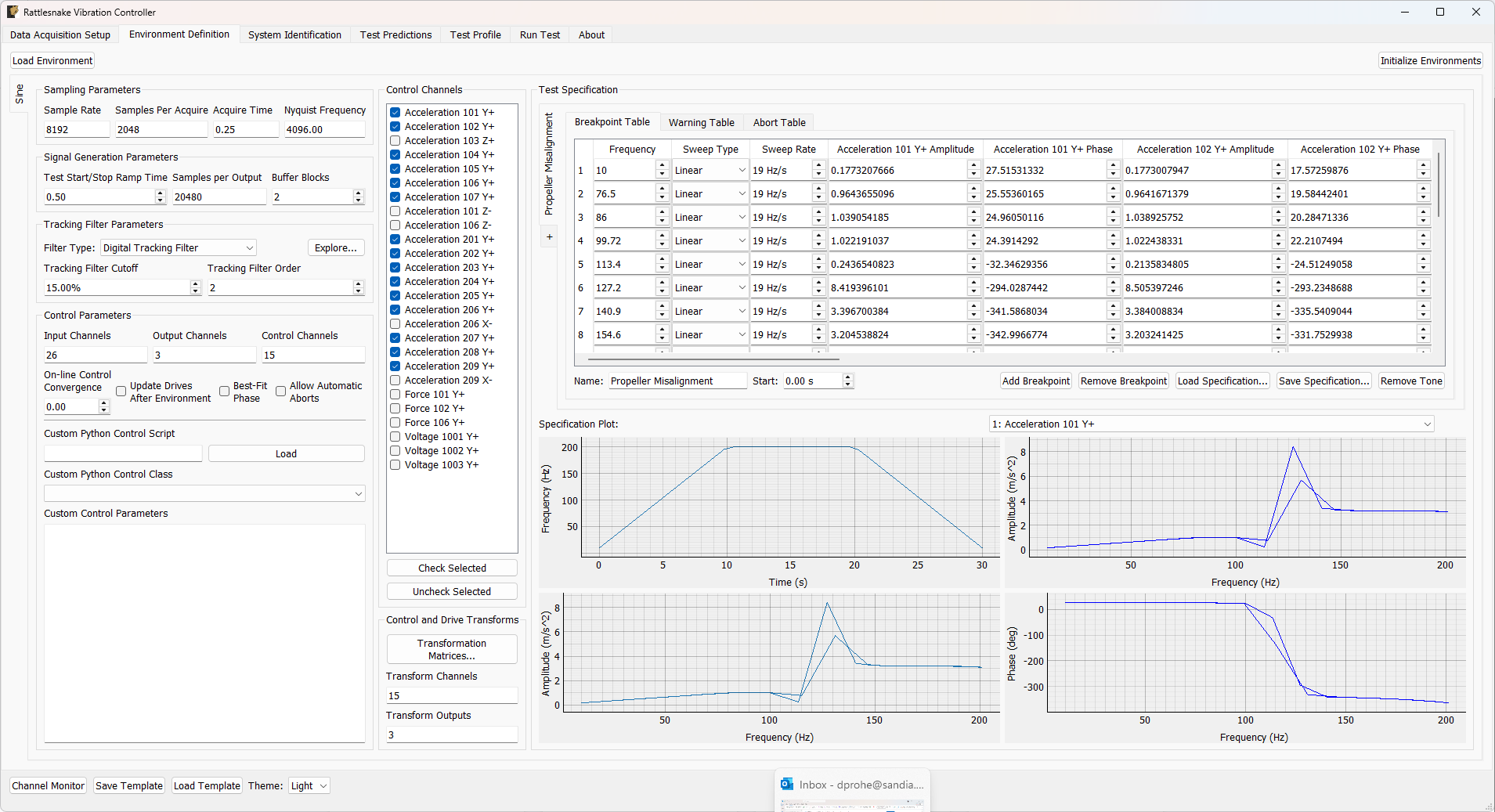
Figure 14.1:UI used to define a MIMO Random Vibration environment.
14.3.1Sampling Parameters
The Sampling Parameters section of the MIMO Sine definition sub-tab consists of the following parameters:
Sample Rate Sample rate in samples per second of the data acquisition hardware. This is a global parameter and must be set in the Data Acquisition Setup tab.
Samples Per Acquire Number of samples that the control process processes at a time. This is driven by the Rattlesnake read buffer size from the data acquisition parameters.
Acquire Time Time to acquire each acquisition chunk in seconds. This is the Samples per Acquire divided by the Sample Rate.
Nyquist Frequency The Nyquist Frequency is the highest frequency that can be analyzed using frequency domain techniques. It is the Sample Rate / 2.
14.3.2Signal Generation Parameters
The Signal Generation Parameters section of the MIMO Sine definition sub-tab consists of the following parameters:
Samples per Output Number of new samples generated by each realization taking into account the overlap with the previous realization.
Test Start/Stop Ramp Time Time in seconds that the controller takes to change the test level to or from zero. The test level is changed smoothly to prevent damaging the excitation hardware or part under test. Larger numbers will result in a more smooth transition between test levels, while smaller numbers will make the test level change more quickly.
Buffer Blocks The number of blocks to keep in the signal generation buffer. A smaller number will make the controller more responsive but also increase the risk of underflow issues which will stop the test abruptly and may damage test hardware.
14.3.3Tracking Filter Parameters
The Tracking Filter Parameters section of the MIMO Sine definition sub-tab consists of properties used to specify the tracking filter, which is used to extract sine-tone information from the measured time histories. Depending on which filter type is selected, different parameters will be made available to the user.
Filter Type The type of filter used to extract the sinusoidal components from the running time data. The Digital Tracking Filter is a less computationally intensive filter, but can struggle to reject noise, other environments, or multiple sine tones. The Overlapped Vold-Kalman filter will do a better job rejecting noise and other environments, and can seamlessly handle multiple overlapping sine tones if they are all defined in this environment. For large tests, the Overlapped Vold-Kalman filter may not be able to be run real-time, which can cause underflow issues as the controller is waiting for its next control decision. It is highly recommended that users use the Explore... button to carefully evaluate their filter parameters and computational complexity!
Explore... Bring up a dialog box allowing the user to explore filter settings for their given test. The user should have their specifications defined prior to clicking this button to ensure filter exploration is performed on the most realistic dataset.
With the digital tracking filter selected, the following parameters are available:
Tracking Filter Cutoff A cutoff in percent of the nominal frequency to use in the digital tracking filter. This value allows the user to specify the trade-off between a faster filter with less noise rejection and a slower filter with more noise rejection.
Tracking Filter Order This value allows the user to specify the order of the filter used in the digital tracking filter.
With the Vold-Kalman filter selected, the following parameters are available:
Vold-Kalman Filter Block Size The Vold-Kalman filter is meant to be run on entire signals and has start and end effects. To transform the Vold-Kalman filter into an on-line filter, an Overlap-and-Add strategy is utilized. This parameter specifies the size of the blocks of data analyzed by each pass of the Vold-Kalman filter.
Vold-Kalman Filter Bandwidth This parameter adjusts the pass-band of the Vold-Kalman filter, which allows the users to specify the trade-off between noise rejection and filter response time.
Vold-Kalman Filter Block Overlap The Vold-Kalman filter is meant to be run on entire signals and has start and end effects. To transform the Vold-Kalman filter into an on-line filter, an Overlap-and-Add strategy is utilized. This parameter specifies the overlap between subsequent measurement frames, aiming to remove the end effects of the filter.
Vold-Kalman Filter Order This value specifies the filter order of the Vold-Kalman filter, which modifies the filter response speed and computational complexity.
If the user is unsure as to which filter they should use, they can use the filter explorer to investigate filter performance, see Section 14.7.4.
14.3.4Control Parameters
The Control Parameters section of the MIMO Sine definition sub-tab consists of properties used to specify the control settings used by the controller. Like other environment types, MIMO Sine allows users to load Python scripts containing custom control laws. Unfortunately, MIMO Sine control laws are by their nature complex, so simple implementations like functions or generators are not available; only class definitions are available. See Section 14.11 for more information on defining a custom control law.
Control Channels A display showing the total number of physical channels this environment is controlling to.
Control Python Script Python script used to specify the control law.
Load Opens a file dialog to load in a Python script containing the control law.
Output Channels A display showing the total number of physical channels this environment is outputting to excitation devices such as vibration shakers.
Input Channels A display showing the total number of physical channels this environment is measuring, including excitation channels and control channels.
Control Python Class Selects the class in the Python script to use as the control law.
Custom Control Parameters Any additional parameters needed by the control law are entered in this text box. It is up to the control law to prescribe what is needed to be defined in this box. The data entered into this box will be passed to the control law as a string to the “extra_parameters” argument. Control laws should parse this string to extract needed information.
On-line Control Convergence A scale factor on the on-line closed loop control. Smaller values will make the controller converge more slowly but may increase stability.
Update Drives After Environment If checked, the initial open-loop drive computation will be updated based on the control achieved during the previous run.
Best-Fit Phase If checked, the absolute phase information will not be controlled to, but rather only the relative phase information between channels. This can be useful if there are time synchronization issues between acquisition and output.
Allow Automatic Aborts If checked, the controller will abort if any abort threshold is reached.
14.3.5Control Channels
The Control Channels section of the MIMO Sine definition sub-tab allows users to select the channels in the environment that will be used for control.
Control Channels Channels that are checked will be used as the control channels for this environment. The control channels should be ordered in the specification the same way they are ordered in this list.
Check Selected When clicked, any selected channels in the Control Channels list will be checked, and therefore used as control channels in the environment.
Uncheck Selected When clicked, any selected channels in the Control Channels list will be unchecked, and therefore not used as control channels in the environment.
14.3.6Control and Drive Transforms
The Control and Drive Transforms section of the MIMO Sine definition sub-tab consists of properties used to specify the response and drive transformations, allowing virtual control degrees of freedom or drive signals to be constructed from physical channels.
Transformation Matrices... Open the transformation matrix dialog to allow specification of transformations to virtual control or virtual excitation channels.
Transform Controls A display showing the number of virtual control channels in the environment due to transformation matrices applied to the physical control channels.
Transform Outputs A display showing the number of virtual excitation channels in the environment due to transformation matrices applied to the physical excitation channels.
Note that if transformation matrices are defined, the number of control channels ends up being the number of rows of the Response Transformation Matrix, rather than the number of physical control channels. The number of physical control channels will be equal to the number of columns of the transformation matrix. The number of control channels in the specification should be equal to the number of rows in the transformation.
See Section 12.8 for more information on specifying transformation matrices.
14.3.7Test Specification
The Test Specification section of the MIMO Sine definition sub-tab consists of properties used to specify the test specification. The main tabs of this section denote the individual sine tones present in this environment. Clicking on the tab labelled + will create a new sine tone. This section also includes four plots to display the specification data in different formats.
Specification Breakpoint Table Frequency breakpoints for the current environment. Use the Tabs to select currently defined sine tones. Clicking the (+) tab will create a new sine tone.
Table Selector Specify the control targets in the Breakpoint Table. Specify warning limits in the Warning Table. Specify abort thresholds in the Abort Table.
Control Channel Selector Select the control channel to visualize in the specification Amplitude and Phase plots.
Specification Amplitude Plot The amplitude of the selected control degree of freedom and sine tone plotted against the frequency.
Specification Phase Plot The phase of the selected control degree of freedom and sine tone plotted against the frequency.
All Amplitudes Plot A plot showing all specified amplitudes against their frequencies.
All Frequencies Plot A plot showing all sine tone frequencies defined in the specification over time.
Within each sine tone, there are three tables behind a sub-tab interface. The Breakpoint Table tab shows the frequency breakpoints, as well as various buttons to add or remove breakpoints.
Breakpoint Table This table allows users to specify the frequency breakpoints for the selected sine tone in the environment. Sweep type and speed between the breakpoints can also be specified, as well as the amplitude and phase targets for each control channel at that breakpoint.
Add Breakpoint Adds a row to the breakpoint table, warning table, and abort tables.
Remove Breakpoint Removes the selected row from the breakpoint, warning, and abort tables.
Load Specification... Opens up a file dialog to load in a specification for this sine tone that was saved outside of Rattlesnake.
Remove Tone Removes this entire sine tone from the test specification.
Name The name used to reference this specific sine tone in the environment.
Start Used to specify the start time of this sine tone, allowing the different tones to start at different times.
The Warning Table contains amplitude limits that will trigger warnings.
Warning Table Define warning thresholds. For each breakpoint, both the warning ampiltude to the left of the breakpoint and to the right of the breakpoint can be specified. This allows users to, for example, set one level below a given breakpoint and a separate level above a given breakpoint.
The Abort Table contains amplitude limits that will trigger aborts.
Abort Table Define abort thresholds. For each breakpoint, both the abort ampiltude to the left of the breakpoint and to the right of the breakpoint can be specified. This allows users to, for example, set one level below a given breakpoint and a separate level above a given breakpoint.
Both warning and abort limit tables allow for specifying the amplitude on the left and right side of the breakpoint independently. This can allow for, for example, looser tolerances during segments of the test that have higher sweep rates. Upper and lower tolerances can also be specified. The warning and abort limits will be shown in the plots along with the breakpoints themselves.
14.4System Identification for the MIMO Sine Environment
When all environments are defined and the Initialize Environments button is pressed, Rattlesnake will proceed to the next phase of the test, which is defined on the System Identification tab.
Before the Sine environment can predict or control the response, it must estimate the transfer function matrix between the drive channels and control channels. This is done through the shared system identification workflow used by the system-ID-based environments.
A typical system identification UI for the sine environment is shown in Figure 14.2.
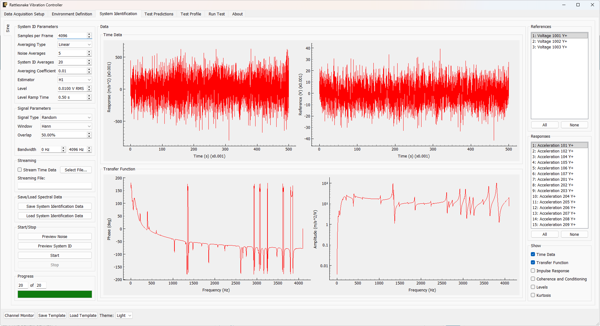
Figure 14.2:System identification UI used by the MIMO Sine environment.
Rattlesnake’s system identification phase will start with a noise floor check, where the data acquisition records data on all the channels without specifying an output signal. After the noise floor is computed, the system identification phase will play out the specified signals to the excitation devices, and transfer functions will be computed using the responses of the control channels to those excitation signals. Section 3.3 describes the System Identification tab and its various parameters and capabilities.
The Sine environment then uses those transfer function to compute initial drive amplitudes and phases.
14.5Test Predictions for the MIMO Sine Environment
Once the system identification is available, the Sine environment can use that information in conjunction with the defined control law to compute initial excitation signals and resulting control responses. The control responses are computed by convolving the excitation signals with the impulse response (the inverse fast Fourier transform of the transfer functions). The specified tracking filters are then used to extract the sine tone amplitudes and phases from the signals. These predictions appear on the Test Predictions tab, shown conceptually in Figure 14.3.
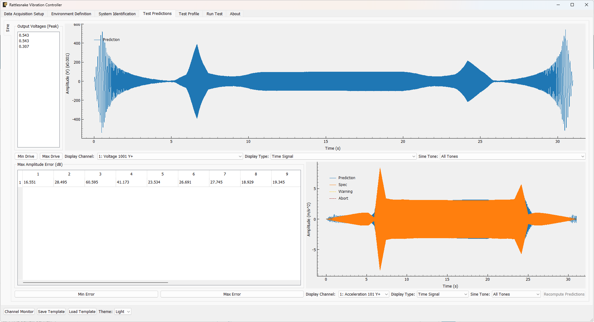
Figure 14.3:Prediction UI used by the MIMO Sine environment.
The prediction UI allows the user to inspect:
predicted excitation time histories, amplitudes, or phases over time or frequency,
predicted filter success in extracting amplitude and phase information from response time histories,
predicted response time histories, amplitudes, or phases over time or frequency,
predicted peak drive voltages,
predicted response errors,
warning and abort threshold comparisons.
The predicted response amplitudes and phases are compared directly against the specification. If time histories are compared, they are compared against time histories synthesized from the specification. Channels that are predicted to violate warning or abort limits are highlighted in the response error matrix.
14.5.1Excitation Prediction
The excitation display on the top portion of the window contains the following displays:
Output Voltages The peak voltages that will be output by the environment based on the open-loop test prediction. Double-clicking an item will show the time history for that drive channel.
Output Plot Displays various quantities of interest related to the excitation signals.
Min Drive Visualize the signal with the smallest peak drive voltage
Max Drive Visualize the drive signal with the largest peak voltage
Output Display Channel Select the drive channel to visualize
Output Display Type Selects the type of data to plot.
Output Sine Tone Selects the sine tone to plot.
Users can plot drive signals, amplitude, and phase quantities over time or frequency. Certain quantities must be plotted on a tone-by-tone basis, while others can be plotted as a superposition of all tones.
14.5.2Response Prediction
Similarly, the response prediction display on the bottom of the window contains the following displays:
Maximum Amplitude Error Table A table showing the maximum amplitude error in decibels for each sine tone (rows) and control channel (columns). Cells highlighted yellow are predicted to hit warning limits while cells highlighted red are predicted to hit abort limits. Double-clicking on a cell will show the amplitude vs. frequency plot for that sine tone and control channel.
Response Prediction Plot Displays various quantities of interest related to the response predictions.
Min Error Visualize the signal with the smallest predicted amplitude error
Max Error Visualize the signal with the largest predicted amplitude error
Recompute Predictions Recompute predictions by running the control law again.
Response Prediction Display Channel Select the control channel to visualize
Response Prediction Display Type Selects the type of data to plot.
Response Prediction Sine Tone Selects the sine tone to plot.
14.6Running the MIMO Sine Environment
The Run Test tab is used to actually run the environment after system identification and prediction are complete.
A typical run page is shown in Figure 14.4.
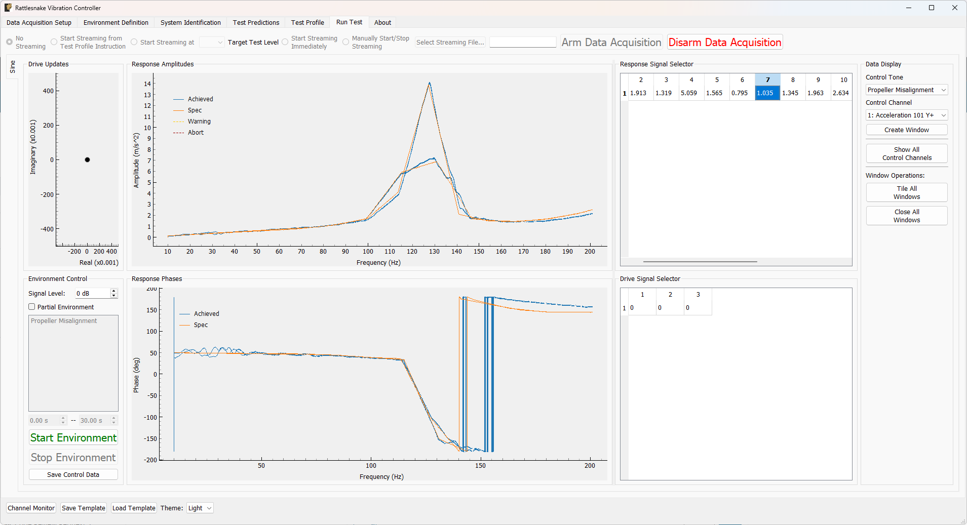
Figure 14.4:Run GUI used by the MIMO Sine environment.
The run page allows the user to:
select test level,
optionally run a partial environment with certain sine tones or certain portions of the sweep time,
monitor achieved response amplitudes and phases,
observe drive updates from the control law,
open plots for individual tones and channels,
and save control data.
14.6.1Drive Updates
The Drive Updates shows the updates that the controller is applying to the open-loop drive signal based on error correction. It is plotted as a complex amplitude, so the phase is encoded as the angle to the -axis, and the amplitude is the distance from the origin. A history of previous drive updates is plotted with lightening colors, so users can identify if the drive updates are diverging.
Drive Updates Shows the updates that the controller is applying to the open-loop drive signal based on error correction. The plot is shown in the complex plane with real part on the horizontal axis and imaginary part on the vertical axis. The drive updates shown correspond to those applied to the selected drive channel and sine tone in the Drive Signal Selector box.
14.6.2Environment Control
The Environment Control allows the user to define how the Sine environment will be run. It contains the following controls:
Signal Level Runs the control at a modified test level. Often used to investigate control accuracy at a lower level without potentially damaging the test article.
Partial Environment If checked, this will enable the user to select only specific sine tones or specific time ranges over which to run the environment, which can be useful to investigate poor control in specific tones or over specific modes of the structure.
Partial Environment Tone Selector Only tones selected in this list will be run if the Partial Environment checkbox is checked.
Partial Environment Start Time If the Partial Environment checkbox is checked, the environment will start at the time specified inthis box.
Partial Environment End Time If the Partial Environment checkbox is checked, the environment will end at the time specified inthis box.
Start Environment Starts the environment controlling to the specified sine tones.
Stop Environment Stops the environment manually.
Save Control Data Saves the current control data from the test.
14.6.3Response Amplitude and Phase
The Response Amplitudes and Response Phases portions of the controller show the amplitude and phase extracted from the channel (column) and sine tone (row) selected in the Response Signal Selector.
Response Amplitude Plot Plots the response amplitude compared to the specification for the selected control channel and sine tone. Additionally plots warning and abort limits if specified.
Response Phase Plot Plots the response phase compared to the specification for the selected control channel and sine tone.
14.6.4Response and Drive Channel Selection
The Response Signal Selector and Drive Signal Selector allow the user to visualize the response amplitude error (in dB) and the drive update amplitude (in dB) respectively. Clicking on a cell in either table will display the data for that sine tone (row) and control or drive channel (column).
Response Signal Selector Shows the decibel error of each control signal (column) and sine tone (row). Selecting a cell will update the signals plotted in the Response Amplitude and Response Phase plots. Cells will be highlighted in yellow if they hit warning limits and highlighted in red if they hit abort limits.
Drive Signal Selector Shows the magnitude of the closed-loop updates applied to the drive signals for each drive signal (column) and sine tone (row). Selecting a cell will display that drive signal and sine tone in the Drive Updates plot.
14.6.5Individual Tone/Channel Displays
The Data Display portion of the Run Test tab allows the user to create new windows showing specific sine tones and channels.
Control Tone Selector Selects the sine tone that will be displayed in the window that is created when the Create Window button is clicked.
Control Channel Selector Selects the control channel that will be displayed in the window that is created when the Create Window button is clicked.
Create Window Create a window to show the signal specified by the selected Control Channel and Control Tone
Show All Control Channels Creates a display window for each control tone and control channel combination in the test and tiles them on the main monitor.
Tile All Windows Tile all open display windows across the main monitor
Close All Windows Closes all existing visualization windows
An example window is shown in Figure 14.5.
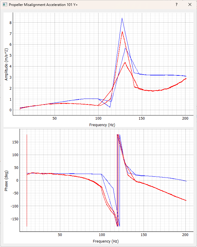
Figure 14.5:A window displaying the amplitude and phase response compared to the specification.
14.7Tracking Amplitude and Phase
A central task in the MIMO Sine environment is the extraction of the instantaneous amplitude and instantaneous phase of the measured response for each control channel and each active sine tone. These extracted quantities are used for:
comparing the achieved response to the specification,
computing warning and abort status,
plotting the achieved response in the Run Test tab,
and updating the complex drive signals during closed-loop control.
Because the Sine environment is deterministic rather than stationary, Rattlesnake does not primarily control to averaged random quantities such as CPSD matrices during a run. Instead, it estimates the response of each active tone directly in the time domain and expresses that response as an amplitude and phase evolving over time.
At a conceptual level, each tracked response component is modeled as
where:
is the instantaneous amplitude,
is the known sinusoidal argument from the frequency breakpoint specification,
is the phase correction required to match the measured response.
The primary filtering problem is therefore to recover and from the measured response , given the known excitation or response reference phase history.
Rattlesnake currently supports two approaches for this task:
a Digital Tracking Filter (DTF), and
an Overlapped Vold-Kalman (VK) Filter.
The DTF is computationally faster and relatively intuitive. The VK filter is more mathematically sophisticated and can provide better discrimination between nearby or crossing sine tones, at the cost of additional computational expense.
14.7.1Digital Tracking Filter
The digital tracking filter operates by demodulating the signal against a known sinusoidal reference and then low-pass filtering the demodulated components.
Suppose the measured signal contains a component of interest whose known instantaneous argument is . Then the measured signal may be projected onto in-phase and quadrature reference signals:
These two signals contain a slowly varying baseband component associated with the desired sine tone, along with higher-frequency content that is rejected by low-pass filtering.
After low-pass filtering, Rattlesnake obtains filtered in-phase and quadrature estimates, which may be denoted and . From these, the instantaneous amplitude and phase are reconstructed as
This is exactly the logic implemented in the digital tracking filter generator used by the Sine environment.
The DTF therefore behaves like a classical synchronous detector followed by a low-pass filter:
the multiplication by sine/cosine translates the tone of interest to baseband,
the low-pass filter removes the higher-frequency terms,
and the baseband complex envelope is converted back to amplitude and phase.
14.7.1.1Tracking Filter Cutoff
The Tracking Filter Cutoff parameter sets the low-pass cutoff as a fraction of the instantaneous tone frequency.
A higher cutoff:
allows faster changes in amplitude and phase to be tracked
rejects noise and neighboring tones less effectively
A lower cutoff:
provides smoother amplitude and phase estimates
responds more slowly to rapid signal changes
14.7.1.2Tracking Filter Order
The Tracking Filter Order parameter sets the order of the Butterworth low-pass filter used after demodulation. Higher-order filters roll off more sharply, which can improve rejection of unwanted content, but may introduce a slower or more oscillatory transient response.
14.7.1.3Digital Tracking Filter Summary
The DTF is generally a good choice when:
tones are well separated,
computational cost must be low,
and rapid online execution is important.
14.7.2Vold-Kalman Filter
The Vold-Kalman Filter 1,2 is a more advanced order tracking method, and includes the method to track multiple sine tones simultaneously. The basic formulation of the VK filter is as follows.
For a given discretely-sampled signal containing primarily a harmonic component, the equation for can be written as
Here is the instantaneous complex amplitude of the sine tone, and is the instantaneous phase or argument of the sine tone. represents an error term. To use the VK filter, we therefore need to know the argument of the sine tone over time; because we can analytically construct the sine sweep frequencies from the breakpoint table in the specification, we can solve for this quantity as the integral of frequency over time. The solution of the VK filter is therefore concerned with the identification of the complex amplitude at each sample for the sine tone, as this will contain instantaneous amplitude and phase of that sine tone, which will be compared to the specified amplitudes and phases to judge test accuracy and perform closed-loop control.
In addition to the data equation (14.10), the VK filter also contains structural equations which describes the mathematical characteristics of the sine tone to be extracted. The goal in this case is that the complex envelope varies slowly over time, at least in comparison to the frequency of the sine tones themselves. Therefore, we can write the structural equation in terms of finite difference operations on the envelope. For first-order, second-order, and third-order filters, these equations are:
In these equations the value represents a small term that allows for the slow modulation of the envelope.
All discrete variables from these equations can be arranged into vectors of length where is the total number of samples.
We can then set up matrix forms for the structural equations (14.18) and data equations (14.19).
where the coefficient matrix is
for the first-order filter or
for the second-order filter, etc. And, the coefficient matrix is a diagonal matrix consisting of the complex argument phasors at each sample in time.
The goal is to minimize the values and , so we can represent the vectors as a scalar product.
The weighted sum of these parameters form the loss function
where is a weighting parameter that determines how heavily the structural equations are weighted compared to the data equations.
The derivative of this function with respect to set to zero gives the minimum of this function.
The solution is then
The above equations are satisfactory for a single tone. However, when multiple tones are simultaneously present in a given signal, we can solve for all tones simultaneously. In this case, the equation for becomes
where now there is a separate complex amplitude and argument for each of the sine tones in the signal.
Following the same logic as above, the function to minimize becomes
The solution is then the for each of the sine tones that minimize this equation. Setting the derivatives to zero gives:
where and is the identity matrix. We also note that due to the phases of the Hermetian diagonal phasor matrices cancelling out when multiplied.
We can assemble this into a large system of equations of the form with
As the matrix has a sparse, banded form, the equation is solved using the sparse solvers in SciPy’s linalg package. Once the envelope is found, it can be split out into the individual complex amplitudes for each sine tone. From these complex amplitudes, the amplitude and phase of the individual sine tones can be derived.
The complex envelope contains the information of interest:
There are a few parameters that can be selected when setting up the VK filter.
14.7.2.1Filter order in the Vold-Kalman method
The Vold-Kalman Filter Order parameter controls the order of the finite-difference smoothness constraint.
Conceptually:
1st order penalizes first differences and favors slowly changing envelopes, using (14.11) for the structural equation,
2nd order penalizes curvature and often gives smoother practical behavior, using (14.12) for the structural equation,
3rd order penalizes higher-order variation and can provide still stronger smoothing, using (14.13) for the structural equation.
Higher order generally increases filter selectivity and mathematical smoothness of the solution at the expense of additional computation.
14.7.2.2Bandwidth in the Vold-Kalman method
The Vold-Kalman Filter Bandwidth controls how narrowly the filter tracks the desired tone.
A smaller bandwidth gives a more selective filter and improves rejection of neighboring tones and broadband noise, but it can make the response slower and may distort rapidly changing amplitude modulation. A larger bandwidth allows faster tracking of amplitude or phase changes but reduces selectivity and can admit contamination from other content. The bandwidth parameter is closely related to the weighting parameter in (14.25), as it controls the tradeoff between smoothness of the solution and matching of the data.
14.7.2.3Multiple simultaneous tones
One of the major advantages of the Vold-Kalman formulation is that multiple sinusoidal components can be solved simultaneously. This is especially important when multiple sine tones exist in the signal and is absolutely necessary if the sine tones cross in frequency.
In these cases, a simple tracking filter may struggle to separate the contributions of the different tones, while the VK formulation can solve for them together as a coupled estimation problem. This is one of the main reasons the Sine environment offers the VK filter as an alternative to the DTF.
14.7.2.4Online and Overlapped Vold-Kalman Filtering
The classical Vold-Kalman filter is most naturally formulated over a full signal block. However, Rattlesnake must use it in an online control environment, where the signal is still being acquired and the control law must update in a timely way.
To make this possible, Rattlesnake implements the VK filter in an overlapped blockwise form.
A blockwise VK solution can exhibit startup and ending transients on each analysis block. If consecutive blocks were simply stitched together end-to-end, these edge effects would become visible in the extracted amplitudes and phases.
To mitigate this, Rattlesnake:
divides the signal into overlapping blocks,
solves the VK problem on each block,
rejects the responses in the overlapped regions, keeping only the “center” portion of each block where the transients are minimal
The Vold-Kalman Filter Block Size sets the number of samples used in each VK solve.
A larger block size generally gives the filter more information, which can remove the effects of startup and ending transients. However, this increases computational cost and decreases controller responsiveness, as the control must acquire more data prior to making a control decision.
The Vold-Kalman Filter Block Overlap sets the overlap fraction between consecutive blocks.
This overlap is used to reduce discontinuities between blocks and to suppress the effect of the VK startup/end transients. In practice, too little overlap can leave visible stitching artifacts due to the startup and ending transients. Increasing overlap improves continuity between blocks; however, it increases redundant computation.
14.7.3Practical Filter Tradeoffs
From a practical standpoint, the DTF and VK filters represent a tradeoff between:
computational cost,
noise rejection,
separation of nearby tones,
transient fidelity,
and robustness for large MIMO tests.
Digital Tracking Filter is often preferable when:
only one tone or well-separated tones are active,
computational budget is limited,
the controller must remain very responsive,
and modest noise rejection is sufficient.
Vold-Kalman Filter is often preferable when:
tones overlap or cross,
better selectivity is required,
the measured response contains significant other-content or noise,
or the user needs more reliable extraction of individual components from a crowded signal.
The DTF is relatively cheap computationally. The VK filter can become expensive, especially because in the Sine environment the filter is applied separately for each control channel. Thus, the total computational burden scales with:
number of control channels,
number of simultaneously active tones,
selected VK block size,
selected overlap,
selected filter order.
For that reason, a filter configuration that is acceptable for a single-channel example may become too expensive for a large multi-channel test.
This is why the filter explorer described in Section 14.7.4 is important: it gives the user the ability to investigate not only the quality of the extracted amplitude and phase, but also the practical computational behavior of the chosen filter.
14.7.4Using the Filter Explorer
The Filter Explorer is accessed by clicking the Explore... button on the Environment Definition tab. This brings up the Filter Explorer dialog box, which is shown in Figure 14.6. The Filter Explorer dialog will take the defined specification and generate a time signal that exactly matches the amplitudes and phases defined for each sine tone in the specification for the selected channel. Noise can also be added to this perfect specification realization to represent realistic test conditions that the filter should reject. The user can then select from filter parameters mirroring those found on the Environment Definition tab described in Section 14.3.3. The filter explorer will then attempt to filter the known signal from the specification, extract amplitude and phase information, and present those data in comparison to the known data from the specification. This allows the user to investigate filter choices prior to running a test.
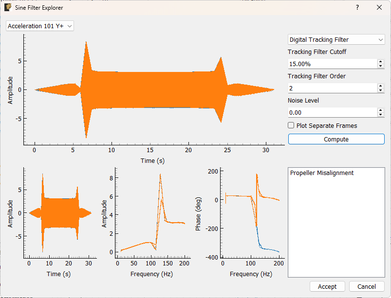
Figure 14.6:The Filter Explorer dialog box that allows users to understand the effect of their tracking filter choices.
Descriptions of the filter selection parameters are found in Section 14.3.3. Additional widgets and displays on the Filter Explorer dialog box include:
Noise Level Simulate noise on the measurements to investigate noise rejection capabilities of the filter.
Plot Separate Frames If selected, the plots will show each frame of data as a separate color so end effects can be more easily identifier. If not selected, a single plot curve will be shown, which is more computationally efficient.
Compute Click this button to start the filter computation.
Full Time History Plot Shows the time history of the control channel including all sine tones in Blue and the sine tones extracted by the filter in Orange. If noise is applied, it is not shown on the desired (Blue) signal, but its effects will be shown on the extracted filter time history (Orange).
Order Time History Plot Shows the time history of the specified sine tone of the chosen control signal in Blue and the corresponding time signal identified by the specified filter parameters in Orange.
Sine Tone Amplitude Plot Plots the amplitude of the specification for the selected control channel and sine tone (Blue) compared to the amplitude extracted from the filtered time signal (Orange) for each frequency.
Sine Tone Phase Plot Plots the phase of the specification for the selected control channel and sine tone (Blue) compared to the phase extracted from the filtered time signal (Orange) for each frequency.
Channel Selector Select the control channel to apply the filter to.
Accept Accepts the specified filter parameters and puts their settings into the Environment Definition user interface.
Cancel Cancels the filter parameter selection and discards any changes made in this dialog box.
14.8Output NetCDF File Structure
Like the other environments in Rattlesnake, the MIMO Sine environment stores its metadata in a netCDF group whose name matches the environment name. This group contains the parameters needed to reconstruct the environment definition, including the sine specifications, the control law configuration, the tracking filter settings, the shared system identification settings, and any transformation matrices.
The root netCDF dataset also contains the global hardware metadata and channel table information described is Section 3.7. The material in this section focuses only on the additional data stored inside the Sine environment’s group.
Because the Sine environment derives from the shared system-identification environment infrastructure, its netCDF group contains both sine-specific fields and shared system-identification fields.
14.8.1NetCDF Dimensions
The Sine environment creates the following dimensions in its netCDF group.
control_channels — the number of physical control channels used by the environment.
response_transformation_rows — the number of rows in the response transformation matrix, if one is defined.
response_transformation_cols — the number of columns in the response transformation matrix, if one is defined.
reference_transformation_rows — the number of rows in the excitation/output transformation matrix, if one is defined.
reference_transformation_cols — the number of columns in the excitation/output transformation matrix, if one is defined.
14.8.2NetCDF Attributes
The following attributes are stored directly on the Sine environment’s netCDF group.
sysid_sample_rate — the sample rate used during system identification.
sysid_frame_size — the number of samples per frame used during system identification.
sysid_averaging_type — the averaging scheme used in the system identification (
LinearorExponential).sysid_noise_averages — the number of frames used in the noise-floor characterization.
sysid_averages — the number of frames used in the transfer-function measurement.
sysid_exponential_averaging_coefficient — the exponential averaging coefficient when exponential averaging is selected.
sysid_estimator — the estimator used for FRF computation, such as H1, H2, H3, or Hv.
sysid_level — the excitation level used during system identification.
sysid_level_ramp_time — the ramp time used to transition into and out of the system identification level.
sysid_signal_type — the signal type used during system identification.
sysid_window — the window applied to the time frames during system identification.
sysid_overlap — the overlap fraction used during system identification.
sysid_burst_on — the fraction of the burst-random frame that is “on,” if burst random is used.
sysid_pretrigger — the fraction of the frame used as pretrigger for burst-random system identification.
sysid_burst_ramp_fraction — the fraction of the burst-random “on” interval used to ramp the burst up and down.
sysid_low_frequency_cutoff — the low-frequency cutoff used during system identification.
sysid_high_frequency_cutoff — the high-frequency cutoff used during system identification.
sample_rate — the sample rate of the environment in samples per second.
samples_per_frame — the number of samples acquired per frame during the run.
ramp_time — the time in seconds used to ramp the environment up from zero or back down to zero.
number_of_channels — the total number of channels in the environment.
update_drives_after_environment — 1 if the open-loop drives should be updated after the environment finishes, 0 otherwise.
phase_fit — 1 if phase fitting is enabled, 0 otherwise.
control_convergence — the scale factor used for the on-line control correction.
allow_automatic_aborts — 1 if the environment is allowed to stop automatically on abort, 0 otherwise.
control_python_script — the path to the Python script containing the custom control law, if one is used.
control_python_class — the class name in the Python script used for the control law, if one is used.
control_python_parameters — additional text parameters passed to the custom control law.
tracking_filter_type — the selected tracking filter type (0 for digital tracking filter, 1 for Vold-Kalman filter).
tracking_filter_cutoff — the cutoff ratio used by the digital tracking filter.
tracking_filter_order — the order of the digital tracking filter.
vk_filter_order — the order of the Vold-Kalman filter.
vk_filter_bandwidth — the bandwidth parameter of the Vold-Kalman filter.
vk_filter_blocksize — the block size used by the blockwise Vold-Kalman implementation.
vk_filter_overlap — the overlap fraction used in the blockwise Vold-Kalman implementation.
buffer_blocks — the number of signal-generation blocks to keep buffered during control.
14.8.3NetCDF Variables
The following variables are stored directly on the Sine environment’s netCDF group.
control_channel_indices — the indices of the physical control channels in the environment. These indices correspond to the physical channels that define the control degrees of freedom before any response transformation is applied. Type: 32-bit integer; Dimensions:
control_channelsresponse_transformation_matrix — the response transformation matrix applied to the physical control channels. This variable is only present if a response transformation matrix is defined. Type: 64-bit float; Dimensions:
response_transformation_rows×response_transformation_colsreference_transformation_matrix — the output/excitation transformation matrix applied to the physical drive channels. This variable is only present if an excitation/output transformation matrix is defined. Type: 64-bit float; Dimensions:
reference_transformation_rows×reference_transformation_cols
14.8.4The specifications Group
A subgroup named specifications is created inside the environment group. Within this group, one subgroup is created for each sine tone in the environment. The subgroup name is the name of the tone as shown in the UI.
For each tone subgroup, the following dimensions are defined:
num_breakpoints — the number of frequency breakpoints in that sine tone.
specification_channels — the number of control channels represented in that tone specification.
two — a helper dimension of size 2 used for warning and abort matrices.
For each sine tone subgroup, the following attribute is stored:
start_time — the start time of that tone in seconds relative to the overall environment.
Each tone subgroup also stores the following variables:
spec_frequency — the frequency breakpoints for the tone. Type: 64-bit float; Dimensions:
num_breakpointsspec_amplitude — the specified amplitude at each breakpoint for each control channel. Type: 64-bit float; Dimensions:
num_breakpoints×specification_channelsspec_phase — the specified phase at each breakpoint for each control channel. These phase values are stored in radians in the netCDF file, even though the external
.npzor.matsine specification files store phase in degrees. Type: 64-bit float; Dimensions:num_breakpoints×specification_channelsspec_sweep_type — the sweep type between adjacent breakpoints. The values correspond to the internal sweep-type representation used by the Sine environment, with
0representing a linear sweep and1representing a logarithmic sweep. The last breakpoint’s stored sweep type is kept for consistency with the full breakpoint table, even though there is no following segment beyond the final breakpoint; this value is effectively ignored. Type: 8-bit integer; Dimensions:num_breakpointsspec_sweep_rate — the sweep rate associated with each breakpoint segment. As with the sweep type, the final row is retained so the saved data matches the internal breakpoint table representation; the value is effectively ignored. Sweep rates are stored in Hz/s for linear sweeps and octaves per minute for logarithmic sweeps. Type: 64-bit float; Dimensions:
num_breakpointsspec_warning — the warning thresholds defined at each breakpoint for each control channel. Type: 64-bit float; Dimensions:
num_breakpoints×two×two×specification_channelsspec_abort — the abort thresholds defined at each breakpoint for each control channel. Type: 64-bit float; Dimensions:
num_breakpoints×two×two×specification_channels
For the warning and abort limits, the meanings of the dimensions are:
first two index:
0= lower warning limit1= upper warning limit
second two index:
0= left side of the breakpoint1= right side of the breakpoint
14.8.5Interpretation of Stored Specification Data
The Sine environment stores the specification in the netCDF4 file in the same logical form as used internally during the run:
frequency-major arrays,
amplitude and phase per control channel,
sweep metadata,
warning and abort breakpoint information,
one subgroup per sine tone.
This is slightly different from the external .mat and .npz sine specification files used when loading individual tones, which are designed to be convenient for exchange with MATLAB or NumPy workflows. In particular:
external specification files store phase in degrees,
internal/netCDF storage uses radians,
and the warning/abort breakpoint arrays are transposed into the controller’s preferred breakpoint-major form.
14.9Saving Control Data
The Sine environment allows saving current control data from the run tab. This occurs when the user clicks the Save Control Data button.
Data is stored to a NumPy Archive (*.npz) file.
This typically includes:
achieved response signals,
achieved amplitudes,
achieved phases,
drive modifications,
frequencies and arguments over time,
target amplitudes and phases.
This data is useful for:
debugging,
offline analysis,
reporting,
or future control-law development.
14.10Using Transformation Matrices
Transformation matrices in the Sine environment behave identically to the the Random Vibration environment. See Section 12.8 for more information.
14.11Writing a Custom Sine Control Law
Unlike the Random Vibration environment, where relatively simple function-based control laws can often be sufficient, the MIMO Sine environment is inherently more stateful. The control logic must manage:
the prescribed response specification as a function of time,
the system identification transfer functions,
the initial open-loop drive synthesis,
the online correction of those drives,
the generation of drive signals in finite blocks,
and optional post-run updates to the drive signal.
For this reason, the Sine environment is built around class-based custom control laws rather than one-shot function calls. A custom Sine control law must therefore be implemented as a Python class with the methods described below. The easiest way to understand the intent of these methods is to compare them to the current default control law, implemented in rattlesnake/environment/sine_sys_id_utilities.py as DefaultSineControlLaw.
A MIMO sine test is not simply a static inversion problem at one frequency. The environment must:
define one or more tones over time,
compute an initial open-loop drive for those tones,
track the achieved response while the test is running,
update the excitation in a stable way,
and generate the output in chunks that match the controller’s block-based acquisition and output architecture.
The control law therefore needs to maintain internal state such as:
the current target amplitudes and phases,
the current preshaped drive amplitudes and phases,
the accumulated drive correction,
write and analysis indices,
and previously sent or measured portions of the signal.
This is why the Sine environment expects a control-law class rather than a simple stateless function.
14.11.1Required Control-Law Lifecycle Methods
A custom Sine control law class is expected to expose the following methods:
__init__(...)system_id_update(...)initialize_control(...)update_control(...)generate_signal(...)finalize_control(...)
The environment calls these methods at different stages of the test.
14.11.1.1__init__(...)
The constructor is called when the environment metadata are initialized and the control law is created. It should store all persistent information required by the control law, including:
specification information,
sample rate,
output oversample,
ramp time,
convergence factor,
buffer sizes,
extra user parameters,
and any system-ID data already available.
The constructor is also a reasonable place to precompute signal representations derived from the specification, such as:
combined time-domain target signals,
per-tone target signals,
breakpoint-derived instantaneous frequencies,
target amplitudes,
target phases.
The current default control law does exactly this. In particular, it uses SineSpecification.create_combined_signals(...) to build:
the total specified response signal,
each tone’s response signal,
the instantaneous frequencies,
the cosine arguments,
the target amplitudes,
and the target phases.
These are stored as persistent arrays so they do not need to be recomputed repeatedly during the run.
14.11.1.2system_id_update(...)
This method is called when the system identification data have been obtained or updated. Its purpose is to convert the system-ID results into a usable open-loop drive estimate.
A custom implementation should use the transfer functions to compute some initial estimate of the drive amplitudes and phases required to reproduce the specified response.
In the default implementation, this method performs the following major steps:
stores the transfer function matrix and related system-ID quantities,
interpolates the FRF pseudoinverse onto the instantaneous frequencies of the specification,
computes the desired complex response
maps that desired response into a complex drive estimate
extracts the resulting drive amplitudes and phases,
reconstructs the corresponding time-domain preshaped drive signals.
This stage is where the default control law solves for the open-loop drive signals that would produce the best estimate of the desired response, assuming the transfer functions are measured exactly.
Any replacement control law must do something equivalent, even if the exact mathematical method differs.
14.11.1.3initialize_control(...)
This method is called at the start of a particular run. It is responsible for initializing the runtime state needed for online control.
Typical responsibilities include:
selecting which tones are active in this run,
selecting the time region of interest,
initializing write and analysis indices,
computing ramp-up and ramp-down portions of the signal,
preparing the first signal block to send to output,
initializing storage for future drive corrections,
resetting any history buffers.
The current default control law uses this method to:
select the controlled tones and time interval,
define ramped portions of both the target and the preshaped drive,
prepare the first portion of the drive signal,
initialize
control_drive_correction,initialize arrays that store sent and achieved signal data.
This method returns the first excitation signal block that will be sent to the output process.
14.11.1.4update_control(...)
This is the key online feedback method. It is called when a new portion of the measured response has been analyzed and reduced to:
tracked time histories,
amplitudes,
phases,
frequencies,
and a time-delay estimate.
A custom control law should compare the achieved response to the target response over the current block and update its internal drive-correction state.
The default implementation does this by:
storing the achieved response data,
identifying the corresponding time block within the full specification,
reconstructing the target complex response over that block,
reconstructing the achieved complex response over that block,
computing the complex error,
projecting that error back through the transfer function pseudoinverse,
scaling the result by a convergence factor,
accumulating the resulting correction into
self.control_drive_correction.
Conceptually, the default implementation is applying a correction of the form
and accumulating this correction across blocks.
Any custom control law that performs closed-loop sine control must implement an analogous update rule, even if the exact form of the correction differs.
14.11.1.5generate_signal(...)
This method is called whenever the signal generation process needs another block of output samples.
It should:
determine the next signal block time range,
retrieve the nominal preshaped excitation over that block,
apply any accumulated corrections,
convert the complex drive representation back into a real time-domain signal,
enforce output limits if needed,
return the next signal block,
and indicate whether the signal generation is complete; there is no more data to generate.
In the default implementation, this method forms a complex excitation signal of the form
and then converts it into a real time signal using cosine reconstruction.
It also applies an optional drive-voltage limit by clipping the magnitude of the complex excitation vector.
This is the method that turns the control law’s internal state into actual samples to be output by the hardware.
14.11.1.6finalize_control(...)
This method is called after the run has completed. It allows the control law to perform any final processing or to prepare updated preshaped drive information for later use.
In the current default implementation, this method primarily returns the current drive signals and associated metadata:
preshaped drive signals,
frequencies,
arguments,
amplitudes,
phases,
ramp sample count.
A more advanced custom implementation could use this stage to:
update future open-loop drives,
compress or archive state,
compute statistics for the UI,
or refine the starting signal for the next run.
14.11.2What the Default Control Law Does
The current DefaultSineControlLaw in sine_sys_id_utilities.py can be understood as having the following stages.
14.11.2.1Stage 1: Parse and store the specification
In __init__, the default control law:
stores the sine specifications,
computes the combined target signals,
computes instantaneous frequency, argument, amplitude, and phase trajectories,
and determines the active tone slices.
This establishes the full target trajectory that the environment will attempt to realize.
14.11.2.2Stage 2: Ingest the system identification results
In system_id_update, the default law:
stores FRFs and related noise/coherence information,
computes the pseudoinverse of the FRF matrix,
interpolates that pseudoinverse onto the tone trajectories,
and computes preshaped drive amplitudes and phases.
This stage generates the initial open-loop estimate of the excitation.
14.11.2.3Stage 3: Build preshaped drive signals
Still within system_id_update, the default implementation reconstructs the corresponding time-domain preshaped drives by applying the amplitude and phase trajectories to the tone arguments.
These preshaped drives are what the environment uses as the baseline excitation before any online correction is applied. This is the signal used to develop the test predictions shown on the Test Predictions tab.
14.11.2.4Stage 4: Initialize runtime control state
In initialize_control, the default control law:
selects the active tones,
defines the run interval,
sets up ramp-up and ramp-down data,
seeds the write and analysis indices,
prepares the first excitation signal block,
and initializes the correction state.
This transitions the control law from an open-loop prediction object into a live online controller.
14.11.2.5Stage 5: Update based on measured response
In update_control, the default implementation:
stores the measured response data,
constructs the target complex response for the current block,
constructs the achieved complex response for the same block,
computes the blockwise complex error,
maps that error back through the interpolated FRF pseudoinverse,
scales the update by the convergence factor,
and accumulates the correction.
This is the core online feedback stage.
14.11.2.6Stage 6: Generate the next output block
In generate_signal, the default control law:
takes the next preshaped excitation block,
adds the accumulated complex correction,
clips amplitudes if a maximum drive limit is configured,
converts the result to a real time-domain drive block,
and returns it.
This continues until all requested signal data have been generated.
14.11.2.7Stage 7: Finalize
In finalize_control, the default law returns the final drive predictions and associated arrays so they can be reused or displayed after the run.
14.11.3What a Custom Sine Control Law Must Do
A replacement control law should preserve the same broad responsibilities, even if the mathematics differ.
At minimum, a custom implementation should be able to:
accept and store specification information,
accept updated system identification results,
compute an initial open-loop drive estimate,
initialize per-run state,
compare achieved response to target response during the run,
compute and accumulate drive corrections,
generate output signal blocks,
optionally finalize or update future drive predictions after the run.
In other words, even if a custom control law uses a completely different control strategy, it still needs to participate correctly in the same lifecycle as the default implementation.
14.11.4Practical Guidance for Implementing a Replacement
14.11.4.1Preserve state explicitly
The Sine control problem is inherently stateful. A custom class should explicitly track:
target signal arrays,
preshaped drive arrays,
current write and analysis indices,
accumulated corrections,
and any other information needed between method calls.
14.11.4.2Be careful about coordinate systems
The control law may be operating on:
physical control channels,
transformed response coordinates,
physical drive channels,
transformed drive coordinates.
A custom implementation should ensure that the transfer functions, specification, and drive outputs are all interpreted in compatible coordinates.
14.11.4.3Respect blockwise execution
The environment acquires and outputs data in finite blocks. A custom control law must therefore be designed to work incrementally, not just as a single full-signal solve.
14.11.4.4Use tracked data, not raw data
By the time update_control(...) is called, the environment has already extracted:
amplitudes,
phases,
frequencies,
and aligned time-domain information.
Most custom control laws should work with those reduced quantities rather than trying to reinterpret the raw time histories from scratch.
14.11.4.5Think carefully about output limits
The default implementation optionally clips the magnitude of the complex excitation to a maximum drive voltage. A replacement control law should decide explicitly:
how actuator saturation is handled,
whether clipping is acceptable,
and what effect that clipping has on stability or convergence.
14.11.5Summary
A custom Sine control law in Rattlesnake is best understood as a stateful object managing the full sine-test lifecycle, not merely as a function that computes one correction.
The default implementation provides a working reference for:
how to convert system ID into initial drives,
how to track achieved response,
how to compute blockwise corrections,
and how to generate real output signals.
When implementing a replacement control law, the most important thing is not to duplicate the exact mathematics of the default implementation, but rather to preserve the required lifecycle:
initialize,
update from system ID,
initialize the run,
update from measured response,
generate output,
finalize.
Any custom control law that satisfies that lifecycle correctly can be integrated into the Sine environment.
- Vold, H., & Leuridan, J. (1995). High Resolution Order Tracking at Extreme Slew Rates Using Kalman Tracking Filters. Shock and Vibration, 2(6), 919402. https://doi.org/10.3233/SAV-1995-2609
- Blough, J. R. (2007). Understanding the Kalman/Vold-Kalman Order Tracking Filters’ Formulation and Behavior. SAE Noise and Vibration Conference and Exhibition, 07NVC-254.