Non-Hierarchical Multifidelity Triangular Maps Tutorial
This notebook is a compact, end-to-end introduction to the NonHierarchicalTriangularMap API. We learn a monotone lower-triangular map \(\widehat{\boldsymbol{S}}^{\mathrm{NH}}\) that pushes a high-fidelity banana target density \(\pi_0\)
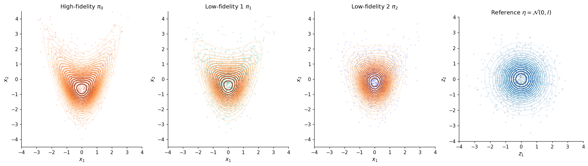
to a standard Gaussian reference \(\eta\). This high-fidelity map is learned using samples from \(\pi_0\) as well as samples from related lower-fidelity densities \(\pi_1\) and \(\pi_2\).
Notation used in this notebook
We use
\(\ell=0\) for the high-fidelity target \(\pi_0\) and
\(\ell=1,\ldots,M\) for lower-fidelity targets. X_ell[ell] represents
\(\mathcal X_\ell=\{x_\ell^{(j)}\}_{j=1}^{N_\ell}\), and S_hat_NH is the learned non-hierarchical map \(\widehat{\boldsymbol{S}}^{\mathrm{NH}}\). Training proceeds in two stages: independently pretrain each low-fidelity \(\widehat{\boldsymbol{S}}_\ell\), then
jointly train the high-fidelity shift \(\delta_k\), scale coefficients
\(\rho_{\ell,k}^{\mathrm{nm}},\rho_{\ell,k}^{\mathrm m}\), and correction
parameters \(\theta_{\ell,k}^{\mathrm{corr}}\). In the API,
shift_order, constant scale_order=0, and correction_order select these
three pieces of the parameterization.
1. Imports and preliminary settings
import time

from IPython.display import Markdown, display
import matplotlib.pyplot as plt
import numpy as np

from mftt import MapParams, OptimizationParams

SEED = 101
rng = np.random.default_rng(SEED)
INPUT_DIM = 2

TARGET_COLOR = "#E76F51"
REFERENCE_COLOR = "#457B9D"
LEARNED_COLOR = "#2A9D8F"
ALTERNATE_COLOR = "#8E5EA2"
MIDDLE_FIDELITY_COLOR = "#43AA8B"
LOW_FIDELITY_COLOR = "#6A77E9"

plt.rcParams.update({
    "figure.dpi": 110,
    "axes.spines.top": False,
    "axes.spines.right": False,
    "axes.labelsize": 11,
    "axes.titlesize": 12,
    "font.size": 10,
})

from mftt import NonHierarchicalMapParams, NonHierarchicalTriangularMap
2. Sampling and density helpers
All helper names, batch conventions, and plotting helpers match the single-fidelity tutorial.
def banana_sample(n_samples, rng, scale_x=1.0, bend=0.5):
    """Draw samples from an analytic banana target."""
    z = rng.standard_normal((n_samples, 2))
    return S_ell_inverse(z, scale_x=scale_x, bend=bend)


def S_ell(x, scale_x=1.0, bend=0.5):
    """Map banana samples to the standard-Gaussian reference."""
    x = np.asarray(x, dtype=float)
    z = x.copy()
    z[:, 0] = x[:, 0] / scale_x
    z[:, 1] = x[:, 1] - bend * (z[:, 0] ** 2 - 1.0)
    return z


def S_ell_inverse(z, scale_x=1.0, bend=0.5):
    """Map standard-Gaussian samples to the banana target."""
    z = np.asarray(z, dtype=float)
    x = z.copy()
    x[:, 0] = scale_x * z[:, 0]
    x[:, 1] = z[:, 1] + bend * (z[:, 0] ** 2 - 1.0)
    return x


def standard_normal_logpdf(z):
    z = np.asarray(z, dtype=float)
    return -0.5 * np.sum(z * z, axis=1) - np.log(2.0 * np.pi)


def banana_logpdf(x, scale_x=1.0, bend=0.5):
    return standard_normal_logpdf(S_ell(x, scale_x=scale_x, bend=bend)) - np.log(scale_x)


def normal_pdf_1d(values, mean=0.0, std=1.0):
    values = np.asarray(values, dtype=float)
    scaled = (values - mean) / std
    return np.exp(-0.5 * scaled * scaled) / (np.sqrt(2.0 * np.pi) * std)


def make_grid(x_limits, y_limits, n=220):
    x1 = np.linspace(*x_limits, n)
    x2 = np.linspace(*y_limits, n)
    xx, yy = np.meshgrid(x1, x2)
    return xx, yy, np.column_stack((xx.ravel(), yy.ravel()))


def style_joint_axis(ax, x_label=r"$x_1$", y_label=r"$x_2$", limits=(-4.0, 4.0, -4.5, 4.5)):
    ax.set(xlabel=x_label, ylabel=y_label, xlim=limits[:2], ylim=limits[2:])
    ax.set_aspect("equal", adjustable="box")
3. Target and reference at a glance
FIDELITY_PARAMS = [
    {"scale_x": 1.05, "bend": 0.65},
    {"scale_x": 0.95, "bend": 0.42},
    {"scale_x": 0.85, "bend": 0.22},
]
FIDELITY_NAMES = ["High-fidelity $\pi_0$", "Low-fidelity 1 $\pi_1$", "Low-fidelity 2 $\pi_2$"]
FIDELITY_COLORS = [TARGET_COLOR, MIDDLE_FIDELITY_COLOR, LOW_FIDELITY_COLOR]

N_ell = [4000, 5000, 6000]
N_test = 6000
N_display = 1500
X_ell = [banana_sample(n, rng, **params) for n, params in zip(N_ell, FIDELITY_PARAMS)]
x_0_test = banana_sample(N_test, rng, **FIDELITY_PARAMS[0])
z_reference_display = rng.standard_normal((N_display, INPUT_DIM))

x_xx, x_yy, x_grid = make_grid((-4.5, 4.5), (-4.5, 4.5))
z_xx, z_yy, z_grid = make_grid((-4.0, 4.0), (-4.0, 4.0))
true_target_densities = [
    np.exp(banana_logpdf(x_grid, **params)).reshape(x_xx.shape)
    for params in FIDELITY_PARAMS
]
reference_density = np.exp(standard_normal_logpdf(z_grid)).reshape(z_xx.shape)

assert np.allclose(
    S_ell_inverse(S_ell(x_0_test[:128], **FIDELITY_PARAMS[0]), **FIDELITY_PARAMS[0]),
    x_0_test[:128],
)
fig, axes = plt.subplots(1, 4, figsize=(17, 4.6), constrained_layout=True)
for axis, density, samples, title, color in zip(
    axes[:3], true_target_densities, X_ell, FIDELITY_NAMES, FIDELITY_COLORS
):
    axis.contour(x_xx, x_yy, density, levels=18, cmap="Oranges")
    axis.scatter(samples[:N_display, 0], samples[:N_display, 1], s=7, alpha=0.22, color=color, edgecolors="none")
    axis.set_title(title)
    style_joint_axis(axis)
axes[3].contour(z_xx, z_yy, reference_density, levels=18, cmap="Blues")
axes[3].scatter(z_reference_display[:, 0], z_reference_display[:, 1], s=7, alpha=0.22, color=REFERENCE_COLOR, edgecolors="none")
axes[3].set_title(r"Reference $\eta=\mathcal{N}(0,I)$")
style_joint_axis(axes[3], r"$z_1$", r"$z_2$", (-4.0, 4.0, -4.0, 4.0))
plt.show()
4. Construct a NH map
Each low-fidelity parent receives its own total-order MapParams; the NH parameters add shift, scale, and correction orders.
optimization = OptimizationParams(
    optimizer="BFGS", reg_cst=1e-10, gtol=1e-8, maxiter=120
)
nhmf_params = NonHierarchicalMapParams(
    low_fidelity_map_params=[
        MapParams(total_order=2, optimization=optimization)
        for _ in range(2)
    ],
    shift_order=2, #\delta_k order
    scale_order=0, # constant scales \rho's
    correction_order=2, # trainable corrections to low-fidelity parents
    optimization=optimization,
)
S_hat_NH = NonHierarchicalTriangularMap(
    [data.copy() for data in X_ell], nhmf_params
)
print(S_hat_NH)
NonHierarchicalTriangularMap(family=non_hierarchical_multifidelity, input_dim=2, low_fidelity_parents=2, corrections=untrained, samples=[4000, 5000, 6000])
5. Train the NH map
The model first pretrains the low-fidelity parents and then trains the coupled HF map with trainable corrections applied to those parent maps.
start = time.perf_counter()
S_hat_NH.train(use_corrections=True, verbose=True)
training_seconds = time.perf_counter() - start
print(f"Non-hierarchical map (S_hat_NH) coefficients: {S_hat_NH.coefficients.flatten().size}")
print(f"Training time: {training_seconds:.2f} s")
print(f"Pretrained low-fidelity maps: {len(S_hat_NH.low_fidelity_maps)}")
Completed training component 1/2.
Completed training component 2/2.
Completed training component 1/2.
Completed training component 2/2.
Training NHMF component 1/2.
Completed NHMF training for component 1.
Training NHMF component 2/2.
Completed NHMF training for component 2.
Non-hierarchical map (S_hat_NH) coefficients: 35
Training time: 8.16 s
Pretrained low-fidelity maps: 2
6. Compare the learned pushforward
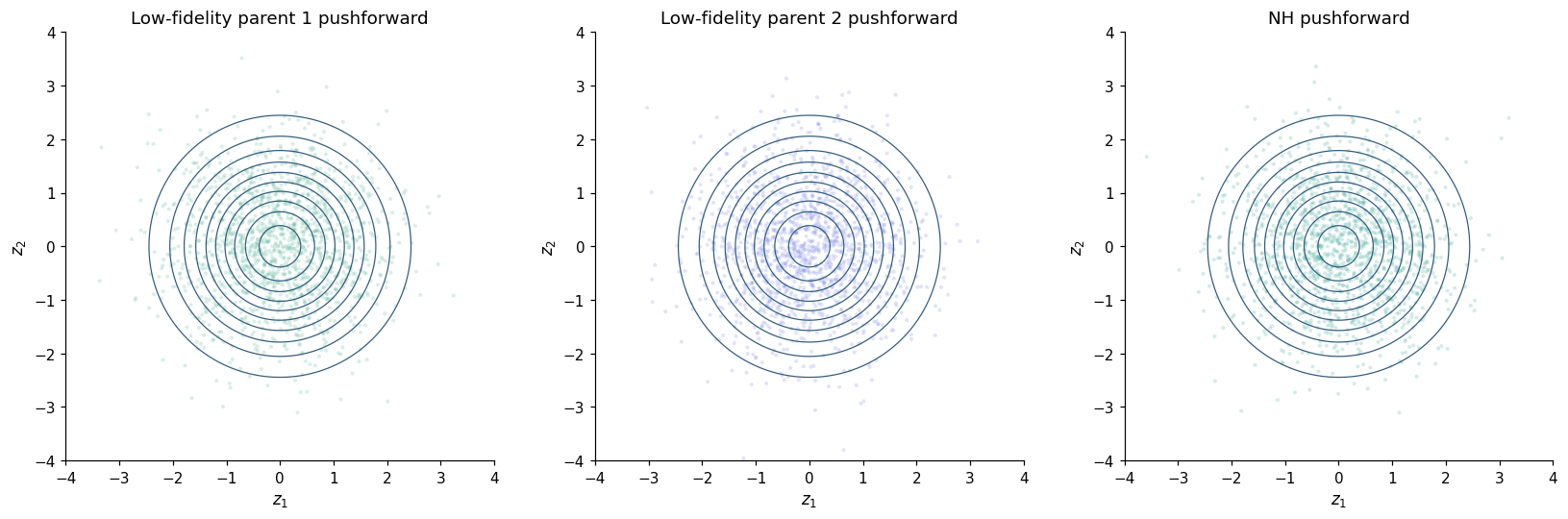
The NH map pushes the high-fidelity target to the Gaussian reference, and each low-fidelity parent map pushes its respective low-fidelity target density to the same Gaussian reference. We show this below.
def map_summary(name, model, elapsed_seconds):
    z_hat = model.evaluate(x_0_test)
    exact_z = S_ell(x_0_test, **FIDELITY_PARAMS[0])
    recovered = model.inverse(z_hat[:512])
    round_trip_error = np.max(np.abs(recovered - x_0_test[:512]))
    assert round_trip_error < 1e-6
    return {"name": name, "coefficients": model.coefficients.flatten().size, "seconds": elapsed_seconds, "S_rmse": float(np.sqrt(np.mean((z_hat-exact_z)**2))), "round_trip_error": float(round_trip_error), "z_hat": z_hat}

summary = map_summary("Non-hierarchical map $\widehat{\boldsymbol{S}}^{\mathrm{NH}}$", S_hat_NH, training_seconds)
print(f"coefficients: {summary['coefficients']}; training: {summary['seconds']:.2f} s")
print(f"RMSE against exact HF transport: {summary['S_rmse']:.4f}")
print(f"max round-trip error: {summary['round_trip_error']:.2e}")
X_ell_test = [banana_sample(N_test, rng, **params) for params in FIDELITY_PARAMS[1:]]
parent_pushforwards = [parent_map.evaluate(samples) for parent_map, samples in zip(S_hat_NH.low_fidelity_maps, X_ell_test)]
fig, axes = plt.subplots(1, 3, figsize=(15, 4.8), constrained_layout=True)
for axis, pushed, title, color in zip(axes, parent_pushforwards + [summary["z_hat"]], ["Low-fidelity parent 1 pushforward", "Low-fidelity parent 2 pushforward", "NH pushforward"], [MIDDLE_FIDELITY_COLOR, LOW_FIDELITY_COLOR, LEARNED_COLOR]):
    axis.contour(x_xx, x_yy, reference_density, levels=10, colors="#315B7D", linewidths=0.8)
    axis.scatter(pushed[:N_display, 0], pushed[:N_display, 1], s=7, alpha=0.2, color=color, edgecolors="none")
    axis.set_title(title)
    style_joint_axis(axis, r"$z_1$", r"$z_2$", (-4.0, 4.0, -4.0, 4.0))
plt.show()
coefficients: 35; training: 8.16 s
RMSE against exact HF transport: 0.0595
max round-trip error: 1.64e-08
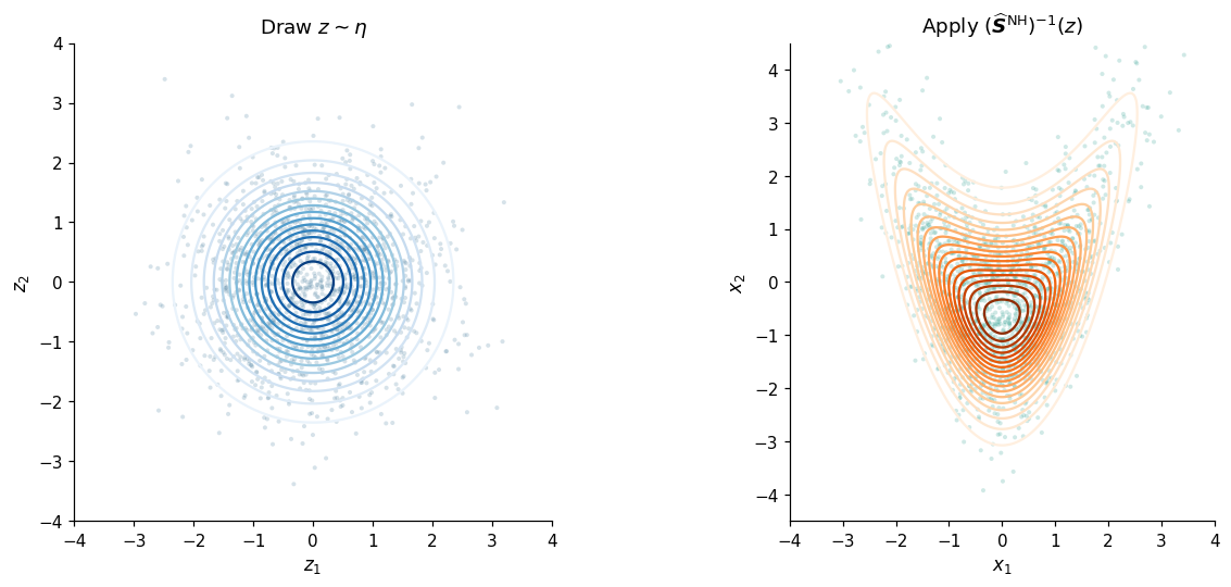
7. Unconditional target sampling via \((\widehat{\boldsymbol{S}}^{\mathrm{NH}})^{-1}\)
N_generate = 5000
sampling_seed = 404
sampling_rng = np.random.default_rng(sampling_seed)
z_draws = sampling_rng.standard_normal((N_generate, INPUT_DIM))
x_draws_from_inverse = S_hat_NH.inverse(z_draws)
x_draws_from_sample = S_hat_NH.sample(N_generate, random_state=sampling_seed)
assert np.allclose(x_draws_from_inverse, x_draws_from_sample)
fig, axes = plt.subplots(1, 2, figsize=(11.5, 4.8), constrained_layout=True)
axes[0].contour(z_xx, z_yy, reference_density, levels=18, cmap="Blues")
axes[0].scatter(z_draws[:N_display, 0], z_draws[:N_display, 1], s=7, alpha=0.22, color=REFERENCE_COLOR, edgecolors="none")
axes[0].set_title(r"Draw $z\sim\eta$")
style_joint_axis(axes[0], r"$z_1$", r"$z_2$", (-4.0, 4.0, -4.0, 4.0))
axes[1].contour(x_xx, x_yy, true_target_densities[0], levels=18, cmap="Oranges")
axes[1].scatter(x_draws_from_inverse[:N_display, 0], x_draws_from_inverse[:N_display, 1], s=7, alpha=0.22, color=LEARNED_COLOR, edgecolors="none")
axes[1].set_title(r"Apply $(\widehat{\boldsymbol{S}}^{\mathrm{NH}})^{-1}(z)$")
style_joint_axis(axes[1])
plt.show()
8. Conditional sampling and conditional density
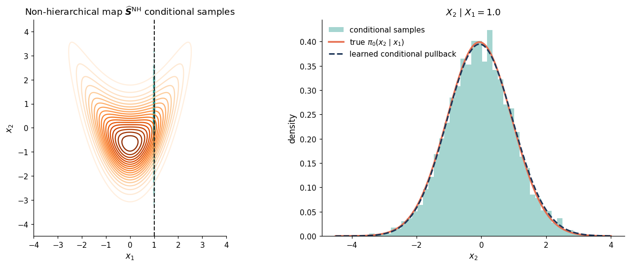
We condition on \(X_1=1.0\) and compare the learned conditional with the analytic HF conditional.
conditioned_x1 = 1.0
N_conditional = 5000
conditional_samples = S_hat_NH.conditional_sample(N_conditional, fixed_indices=[0], fixed_values=np.array([conditioned_x1]), random_state=808)
assert np.allclose(conditional_samples[:, 0], conditioned_x1)
x2_conditional_grid = np.linspace(-4.5, 4.0, 500)
conditional_grid = np.column_stack((np.full_like(x2_conditional_grid, conditioned_x1), x2_conditional_grid))
true_conditional_mean = FIDELITY_PARAMS[0]["bend"] * ((conditioned_x1 / FIDELITY_PARAMS[0]["scale_x"]) ** 2 - 1.0)
true_pi_0_conditional_density = normal_pdf_1d(x2_conditional_grid, mean=true_conditional_mean)
learned_pi_0_conditional_logdensity = S_hat_NH.conditional_pullback_logpdf(conditional_grid, fixed_indices=[0])
learned_pi_0_conditional_density = S_hat_NH.conditional_pullback_pdf(conditional_grid, fixed_indices=[0])
assert np.all(np.isfinite(learned_pi_0_conditional_logdensity))
assert np.all(np.isfinite(learned_pi_0_conditional_density)) and np.all(learned_pi_0_conditional_density >= 0.0)
fig, axes = plt.subplots(1, 2, figsize=(12, 4.8), constrained_layout=True)
axes[0].contour(x_xx, x_yy, true_target_densities[0], levels=18, cmap="Oranges")
axes[0].scatter(conditional_samples[:N_display, 0], conditional_samples[:N_display, 1], s=8, alpha=0.2, color=LEARNED_COLOR, edgecolors="none")
axes[0].axvline(conditioned_x1, color="#222222", linestyle="--", linewidth=1.4)
axes[0].set_title(r"Non-hierarchical map $\widehat{\boldsymbol{S}}^{\mathrm{NH}}$ conditional samples")
style_joint_axis(axes[0])
axes[1].hist(conditional_samples[:, 1], bins=45, density=True, alpha=0.42, color=LEARNED_COLOR, edgecolor="none", label="conditional samples")
axes[1].plot(x2_conditional_grid, true_pi_0_conditional_density, color=TARGET_COLOR, linewidth=2.3, label=r"true $\pi_0(x_2\mid x_1)$")
axes[1].plot(x2_conditional_grid, learned_pi_0_conditional_density, color="#1D3557", linestyle="--", linewidth=2.0, label="learned conditional pullback")
axes[1].set(title=rf"$X_2\mid X_1={conditioned_x1}$", xlabel=r"$x_2$", ylabel="density")
axes[1].legend(frameon=False)
plt.show()
9. The map-induced joint target density
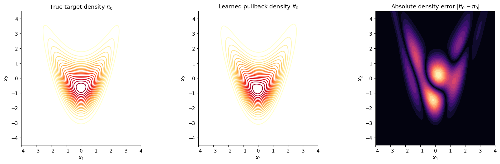
pullback_pdf(x) evaluates \(\widehat\pi_0(x)=\eta(\widehat{\boldsymbol{S}}^{\mathrm{NH}}(x))|\det\nabla\widehat{\boldsymbol{S}}^{\mathrm{NH}}(x)|\).
learned_pi_0_logdensity = S_hat_NH.pullback_logpdf(x_grid)
learned_pi_0_density = S_hat_NH.pullback_pdf(x_grid).reshape(x_xx.shape)
assert np.all(np.isfinite(learned_pi_0_logdensity))
assert np.all(np.isfinite(learned_pi_0_density)) and np.all(learned_pi_0_density >= 0.0)
absolute_density_error = np.abs(learned_pi_0_density - true_target_densities[0])
density_max = max(true_target_densities[0].max(), learned_pi_0_density.max())
density_levels = np.linspace(0.0, density_max, 20)[1:]
fig, axes = plt.subplots(1, 3, figsize=(15.5, 4.7), constrained_layout=True)
for axis, density, title in zip(axes[:2], [true_target_densities[0], learned_pi_0_density], [r"True target density $\pi_0$", r"Learned pullback density $\widehat\pi_0$"]):
    axis.contour(x_xx, x_yy, density, levels=density_levels, cmap="YlOrRd")
    axis.set_title(title)
    style_joint_axis(axis)
axes[2].contourf(x_xx, x_yy, absolute_density_error, levels=18, cmap="magma")
axes[2].set_title(r"Absolute density error $|\widehat\pi_0-\pi_0|$")
style_joint_axis(axes[2])
plt.show()
10. Math-to-API summary
Task |
Mathematical operation |
|
|---|---|---|
Configure peer parents and correction orders |
parent maps plus coupled shift/scale/correction blocks |
|
Train with parent corrections |
pretrained parents plus trainable corrections applied to them |
|
Push target samples to reference |
\(\widehat{\boldsymbol{S}}^{\mathrm{NH}}(x)\) |
|
Pull reference samples to target |
\((\widehat{\boldsymbol{S}}^{\mathrm{NH}})^{-1}(z)\) |
|
Draw unconditional target samples |
sample reference, then invert |
|
Draw \(X_2\mid X_1=a\) |
clamp a leading coordinate while inverting |
|
Evaluate learned densities |
change of variables |
|