Hierarchical multifidelity maps

Hierarchical multifidelity transport replaces one difficult high-fidelity transport with a composition of simpler stage maps. This page develops the two hierarchical formulations implemented by HierarchicalTriangularMap and then connects each mathematical object to the library.

The basic target-to-reference convention and pullback notation are reviewed in the notation guide. The single-fidelity guide develops the monotone stage-map parameterization and its two training paths. Here, the prescribed reference is \(\eta=\mathcal N(0,I)\).

Ordered fidelity data

Let \(\pi_\ell\) denote the target density at fidelity \(\ell\). For the hierarchical methods, MFTT requires the user to specify a fidelity ordering

\[ \pi_M \longrightarrow \pi_{M-1} \longrightarrow \cdots \longrightarrow \pi_0, \]

where the arrows point toward increasing fidelity: \(\pi_0\) is the high-fidelity target and \(\pi_M\) is the lowest-fidelity target. For each level, the available dataset is

\[ \mathcal X_\ell =\{\boldsymbol{x}_\ell^{(j)}\}_{j=1}^{N_\ell}, \qquad \boldsymbol{x}_\ell^{(j)}\sim\pi_\ell. \]

The datasets need not be paired and may contain different numbers of samples, but they must have the same coordinate dimension. Supply them in high-to-low order as [X_0, ..., X_M]. The hierarchy is user specified; MFTT does not infer or reorder the fidelity levels.

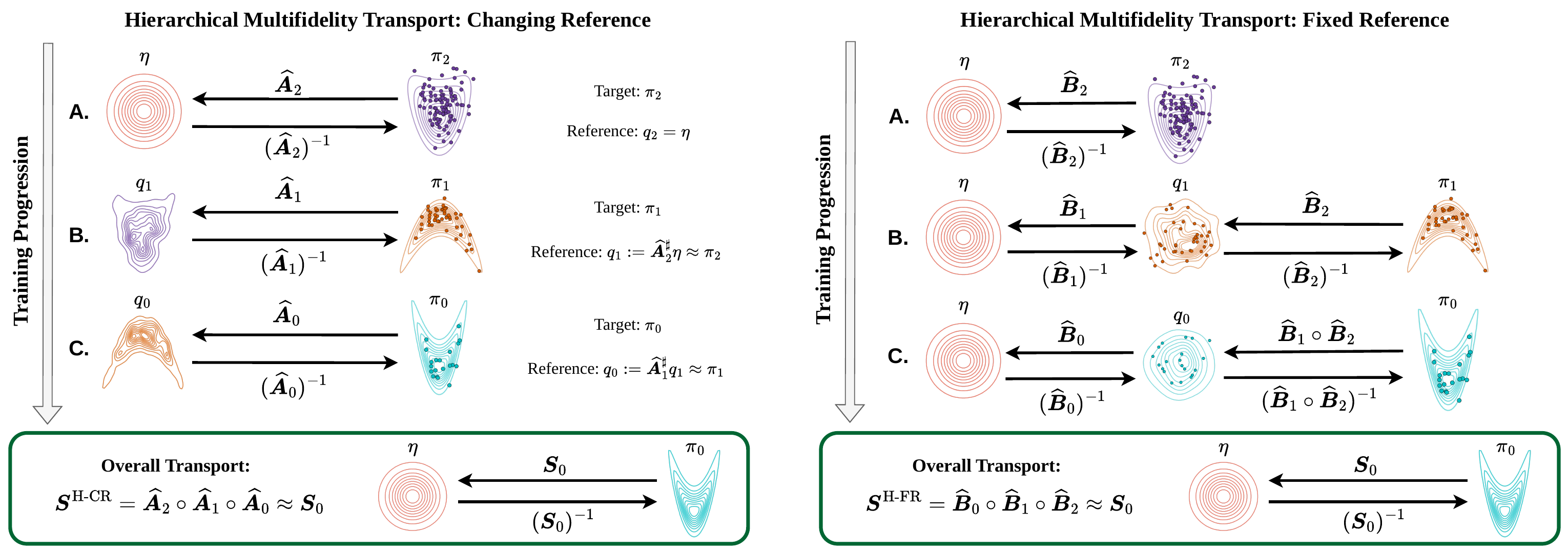
Tri-fidelity changing-reference (left) and fixed-reference (right) constructions. The upper rows proceed from low- to high-fidelity training; left-pointing arrows are learned target-to-reference maps and right-pointing arrows are their inverses. The bottom row shows the final transport from \(\pi_0\) to \(\eta\).

The two formulations differ in what changes at each stage:

Property	Changing reference	Fixed reference
Stage reference	Map-induced \(q_\ell\)	Standard normal \(\eta\)
Stage data	Samples from \(\pi_\ell\)	Samples transformed by lower-fidelity maps
Stage interpretation	Transport toward the adjacent lower fidelity	Residual correction to a cumulative transport
Final composition	\(\widehat A_M\circ\cdots\circ\widehat A_0\)	\(\widehat B_0\circ\cdots\circ\widehat B_M\)
Forward evaluation order	\(0,1,\ldots,M\)	\(M,M-1,\ldots,0\)
Optimization structure	Generally coupled after the first stage	Componentwise with Gaussian \(\eta\)
Most suitable when	Adjacent-fidelity transports are simple	Lower-fidelity maps leave simple residuals

Both methods train stages from the lowest fidelity to the highest, \(\ell=M,M-1,\ldots,0\).

Changing-reference hierarchy

Formulation

The ideal changing-reference decomposition is

\[ \boldsymbol S_0 =\boldsymbol A_M\circ\boldsymbol A_{M-1}\circ\cdots\circ\boldsymbol A_0. \]

The lowest-fidelity map sends \(\pi_M\) to \(\eta\). Every subsequent map mimics a transport between adjacent fidelity levels: \(\boldsymbol A_\ell\) sends \(\pi_\ell\) toward \(\pi_{\ell+1}\).

In the learned construction, initialize \(q_M:=\eta\). At stage \(\ell\), train a triangular map such that

\[ (\widehat{\boldsymbol A}_\ell)_\sharp\pi_\ell\approx q_\ell. \]

For \(\ell=M,M-1,\ldots,1\), its pullback becomes the reference for the next higher-fidelity stage:

\[ q_{\ell-1} :=\widehat{\boldsymbol A}_\ell^{\sharp}q_\ell, \qquad q_{\ell-1}(\boldsymbol x) =q_\ell(\widehat{\boldsymbol A}_\ell(\boldsymbol x)) \left|\det\nabla\widehat{\boldsymbol A}_\ell(\boldsymbol x)\right|. \]

Thus \(q_{\ell-1}\approx\pi_\ell\). The final learned map is

\[ \widehat{\boldsymbol S}^{\mathrm{H\text{-}CR}} :=\widehat{\boldsymbol A}_M\circ\widehat{\boldsymbol A}_{M-1} \circ\cdots\circ\widehat{\boldsymbol A}_0 \approx\boldsymbol S_0. \]

Stagewise training

Given \(q_\ell\) and \(\mathcal X_\ell\), stage \(\ell\) minimizes

\[ \min_{\boldsymbol\theta_\ell} \frac{1}{N_\ell}\sum_{j=1}^{N_\ell} \left[ -\log q_\ell\!\left( \widehat{\boldsymbol A}_\ell( \boldsymbol x_\ell^{(j)};\boldsymbol\theta_\ell) \right) -\log\det\nabla\widehat{\boldsymbol A}_\ell( \boldsymbol x_\ell^{(j)};\boldsymbol\theta_\ell) \right] +\lambda_\ell^A\lVert\boldsymbol\theta_\ell\rVert_2^2. \]

For a tri-fidelity hierarchy, the procedure is:

1. Train \(\widehat{\boldsymbol A}_2\) on \(\mathcal X_2\) against \(q_2=\eta\), then set \(q_1=\widehat{\boldsymbol A}_2^\sharp q_2\).

2. Train \(\widehat{\boldsymbol A}_1\) on \(\mathcal X_1\) against \(q_1\), then set \(q_0=\widehat{\boldsymbol A}_1^\sharp q_1\).

3. Train \(\widehat{\boldsymbol A}_0\) on \(\mathcal X_0\) against \(q_0\).

4. Evaluate a high-fidelity point by applying \(\widehat{\boldsymbol A}_0\), then \(\widehat{\boldsymbol A}_1\), then \(\widehat{\boldsymbol A}_2\).

After the lowest-fidelity stage, \(q_\ell\) is map induced and need not be Gaussian, log-concave, or factorized. The component objectives are therefore generally coupled. MFTT uses the all-at-once analytic-gradient training path (TriangularMap.train_aao) for every changing-reference stage. This method faithfully models adjacent transports, but recursive reference evaluation can make it more expensive and harder to optimize. Indeed, with few exceptions, we recommend using the fixed-reference hiearchical method presented below. Empirically, it is both faster to train and more stable.

Fixed-reference hierarchy

Formulation

The fixed-reference construction keeps \(\eta\) at every stage and transforms the data instead. Its ideal composition is

\[ \boldsymbol S_0 =\boldsymbol B_0\circ\boldsymbol B_1\circ\cdots\circ\boldsymbol B_M. \]

At the lowest fidelity, set \(\boldsymbol y_M^{(j)}:=\boldsymbol x_M^{(j)}\). For each \(\ell=M-1,M-2,\ldots,0\), transform the current dataset through every map already learned at lower fidelities:

\[ \boldsymbol y_\ell^{(j)} := \left( \widehat{\boldsymbol B}_{\ell+1}\circ \widehat{\boldsymbol B}_{\ell+2}\circ\cdots\circ \widehat{\boldsymbol B}_M \right)(\boldsymbol x_\ell^{(j)}). \]

If the lower-fidelity composition already sends \(\pi_\ell\) close to \(\eta\), then \(\widehat{\boldsymbol B}_\ell\) only needs to learn the remaining residual correction. Each stage solves

\[ \min_{\boldsymbol\theta_\ell} \frac{1}{N_\ell}\sum_{j=1}^{N_\ell} \left[ -\log\eta\!\left( \widehat{\boldsymbol B}_\ell( \boldsymbol y_\ell^{(j)};\boldsymbol\theta_\ell) \right) -\log\det\nabla\widehat{\boldsymbol B}_\ell( \boldsymbol y_\ell^{(j)};\boldsymbol\theta_\ell) \right] +\lambda_\ell^B\lVert\boldsymbol\theta_\ell\rVert_2^2. \]

The resulting transport is

\[ \widehat{\boldsymbol S}^{\mathrm{H\text{-}FR}} :=\widehat{\boldsymbol B}_0\circ\widehat{\boldsymbol B}_1 \circ\cdots\circ\widehat{\boldsymbol B}_M \approx\boldsymbol S_0. \]

Stagewise training

For a tri-fidelity hierarchy, the procedure is:

1. Train \(\widehat{\boldsymbol B}_2\) on \(\mathcal X_2\) against \(\eta\).

2. Form \(\boldsymbol y_1=\widehat{\boldsymbol B}_2(\boldsymbol x_1)\) and train \(\widehat{\boldsymbol B}_1\) on those transformed samples against \(\eta\).

3. Form \(\boldsymbol y_0=(\widehat{\boldsymbol B}_1\circ \widehat{\boldsymbol B}_2)(\boldsymbol x_0)\) and train \(\widehat{\boldsymbol B}_0\) against \(\eta\).

4. Evaluate a high-fidelity point in that same map order: \(\widehat{\boldsymbol B}_2\), then \(\widehat{\boldsymbol B}_1\), then \(\widehat{\boldsymbol B}_0\).

Because every stage uses the factorized standard-Gaussian reference, MFTT uses the componentwise TriangularMap.train path. Fixed-reference training is therefore usually faster and more stable than changing-reference training.

From the equations to MFTT

Assume X_0, X_1, and X_2 are two-dimensional NumPy arrays whose rows are samples. Configure one MapParams object per fidelity, in the same high-to-low order as the data:

from mftt import (
    HierarchicalMapParams,
    HierarchicalTriangularMap,
    MapParams,
    OptimizationParams,
)

X_ell = [X_0, X_1, X_2]
optimization = OptimizationParams(
    optimizer="BFGS", reg_cst=1e-8, gtol=1e-6, maxiter=200
)
hierarchical_params = HierarchicalMapParams(
    fidelity_map_params=[
        MapParams(total_order=2, optimization=optimization)
        for _ in X_ell
    ]
)

# Use separate objects to retain both trained compositions.
changing = HierarchicalTriangularMap(X_ell, hierarchical_params)
fixed = HierarchicalTriangularMap(X_ell, hierarchical_params)

changing.train(method="changing_reference")
fixed.train(method="fixed_reference")

z_changing = changing.evaluate(X_0[:32])
z_fixed = fixed.evaluate(X_0[:32])
x_draws = fixed.sample(1000)

print(changing.evaluation_order)  # [0, 1, 2]
print(fixed.evaluation_order)     # [2, 1, 0]

The configurations may use different basis orders or regularization at each fidelity. Passing optimization=... directly to train instead applies one optimizer configuration to every stage. The reg_cst field is the code-level counterpart of \(\lambda_\ell^A\) or \(\lambda_\ell^B\).

Mathematical object	Library representation
\(\mathcal X_\ell\)	model.train_data[ell] (raw data) and model.standardized_train_data[ell]
\(\widehat A_\ell\) or \(\widehat B_\ell\)	model.stages[ell].map
Changing-reference \(q_\ell\)	model.stages[ell].reference
Fixed-reference transformed samples \(\boldsymbol y_\ell\)	model.stages[ell].stage_train_data
Stage coefficients \(\boldsymbol\theta_\ell\)	model.coefficients.stages[ell]
Regularization \(\lambda_\ell^A\) or \(\lambda_\ell^B\)	OptimizationParams.reg_cst in the corresponding MapParams
Final target-to-reference composition	model.evaluate(x)
Inverse composition	model.inverse(z) or model.sample(n)
Forward stage order	model.evaluation_order

Internal standardization and inspection

MFTT independently standardizes each fidelity dataset before stage training. The stage maps themselves then use identity standardization, so all stage compositions act in standardized coordinates. Public methods accept and return raw high-fidelity coordinates: evaluate applies the high-fidelity standardization, while inverse, sampling, and density methods undo or account for it.

After training:

• stages[ell] contains the fidelity index, configuration, raw data, actual stage training data, reference, and trained stage map.

• stages and maps remain in fidelity order [0, ..., M]; use evaluation_order to determine composition order.

• partial_evaluations(x) returns the high-fidelity-standardized input and the state after every stage in evaluation order.

• Calling train again resets all stage maps and replaces the previous fit. Create separate objects when comparing the two methods.

For a complete executable tutorial, continue to the hierarchical notebook. See the hierarchical API reference for all methods and shared operations for inversion, conditional sampling, and density evaluation.