MIMO Drive Prediction with Response Limiting

This notebook demonstrates how ForceFinder can be used for shaker drive prediction in MIMO random vibration testing with response limiting. This example uses the beam system that was developed here with a random vibration specification that is developed from a single DOF vibration specification in MIL-STD 810H. An image of the beam system is shown below, the blue arrows (the straight arrows above the beam) are the control DOFs for the vibration test, the red arrows (below the beam) are the excitation DOFs, and the yellow arrows (the curved arrows above the beam) are the DOFs with response limits.

Note

The straight arrows indicate a translating DOF and the curved arrows indicate a rotating DOF. The nodes are labeled 101-109 from left to right. The translating direction on the beam (vertical on the page) is Z+ and the rotating direction is RY+.

The example data for this beam system is generated using the following process:

1. The SDynPy System object for the beam is imported

2. FRFs are computed for the beam system using the frequency_response method for the beams System object

3. A CPSD specification is made from a single DOF vibration specification from MIL-STD 810H

4. Response limits will be defined with a ResponseLimit object

import sdynpy as sdpy
import forcefinder as ff
import numpy as np
import matplotlib.pyplot as plt

No GPU Found, Geometry plotting will not work!

beam_system = sdpy.System.load(r'./example_system/example_system.npz')

Computing the FRFs

The FRFs are computed using a bandwidth of 5-500 Hz (which matches the specification that is defined below) and a frequency resolution 1 Hz. The displacement derivative is set to two, meaning the the FRFs are in accelerance format. The ordinate of the FRFs is divided by 9.81 to convert the FRFs from SI units to SI-G units (acceleration in Gs).

Note

The FRFs are computed in acceleration/force units, based on limitations of the model. This is being used as an analog for the acceleration/voltage units that are common in MIMO vibration testing.

frf_frequency = np.arange(496)+5
drive_coordinate = sdpy.coordinate_array(node=[102,104,106,108], direction=3)

frfs = beam_system.frequency_response(frf_frequency,
                                      references=drive_coordinate, 
                                      displacement_derivative=2)
frfs.ordinate /= 9.81

Specification

The specification for this example is based off the unknonwn orientation “common carrier (US highway truck vibration exposure)” single DOF vibration specification that is defined in method 514.8, annex C of MIL-STD 810H. This example problem is treating the beam as a shaker table, where the goal is to control the beam as a rigid body. The rigid behavior is specified by applying same single axis specification PSD to each control DOF. The cross-terms for the specification CPSD is defined by a coherence 0.9 between each DOF and zero phase between each DOF.

Note

The approach of applying a single axis vibration specification equally to all the control DOFs is for demonstration purposes only and should not be treated as an endorsement of the method.

The specification from MIL-STD 810H is provided as a set of PSD breakpoints, which must be converted to a narrow band PSD before it can be turned into a MIMO specification. This conversion is done using log-log interpolation on the frequency axis.

breakpoint_frequencies = [5,     40,    120,      121,   200,   240,    266,      500]
breakpoint_amplitudes =  [0.015, 0.015, 0.002025, 0.003, 0.003, 0.0015, 0.000475, 0.00015]

narrowband_specification = 10**(np.interp(np.log10(frf_frequency), 
                                          np.log10(breakpoint_frequencies), 
                                          np.log10(breakpoint_amplitudes)))

The coherence and phase for the specification are manually defined. Note that several extra steps are used in this code block to shape the arrays for the necessary operations.

specification_psd = narrowband_specification[...,np.newaxis]*np.array(([[1,1,1,1]]*frf_frequency.shape[0]))

specification_phase = np.zeros((frf_frequency.shape[0],4,4), dtype=float)

specification_coherence = np.ones((4,4), dtype=float)*0.9
np.fill_diagonal(specification_coherence, 1)
specification_coherence = np.broadcast_to(specification_coherence[np.newaxis,...], 
                                          (frf_frequency.shape[0],4,4))

The PSDs, coherence, and phase are used to generate the full specification CPSD matrix for the simulated MIMO test using the cpsd_from_coh_phs function in SDynPy. The specification CPSD is initially generated as an ndarray in specification_cpsd. This ndarray is then populated into a SDynPy PowerSpectralDensityArray in specification.

specification_dofs = sdpy.coordinate_array(node=[102,104,106,108], direction=3)

specification_cpsd = sdpy.signal_processing.cpsd.cpsd_from_coh_phs(specification_psd, 
                                                                specification_coherence, 
                                                                specification_phase)

specification = sdpy.power_spectral_density_array(frf_frequency, 
                                                  np.moveaxis(specification_cpsd,0,-1),
                 sdpy.coordinate.outer_product(specification_dofs, specification_dofs))

Defining the Limit

Limits for the different DOFs are defined below in a ResponseLimit object, which contains all the limits for the simulated MIMO test. This example shows one way to define the ResponseLimit object, refer to the API documentation for more details.

Note

Contrived limits are used here to limit the rotation of the beam. The breakpoint frequencies and amplitudes were chosen to demonstrate the flexibility of the ResponseLimit object and ensure that the limits would effect the estimated drives.

Tip

Response limits do not need to be defined for the full test bandwidth and a different number of breakpoints can be used for the different limits in the object. The main requirement for using a ResponseLimit object is that FRF data must exist to predict the response PSDs at the limit DOFs.

example_limit = ff.ResponseLimit(limit_coordinate=['105RY+', '107RY+'],
                            breakpoint_frequency=[[200, 400], # 105RY+
                                                [50, 150, 250, 280, 500]], # 107RY+
                            breakpoint_level=[[0.03, 0.03], # 105RY+
                                            [0.1, 0.5, 1, 0.01, 0.01]]) # 107RY+

Creating the SPR Object without a Response Limit

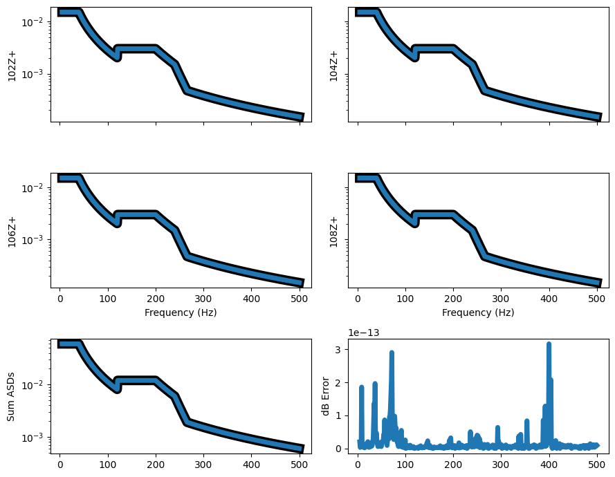
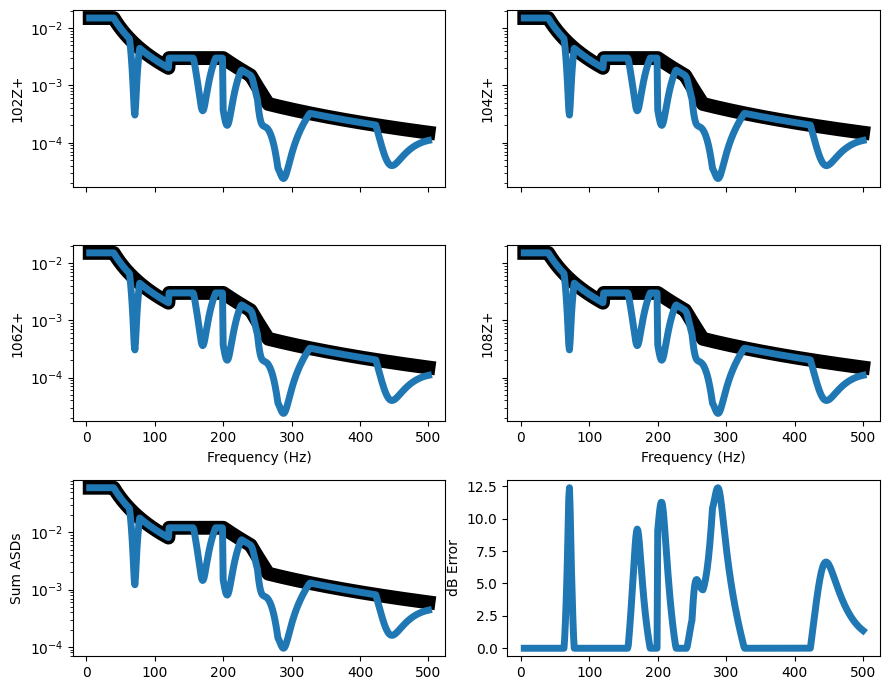
This section creates the basic SPR object and estimates the drives with the pseudo-inverse method without enforcing the response limits. The control accuracy is evaluated using the error_summary method, which shows that the PSDs are controlled with line-on-line accuracy. Although it is not shown here, the phase and coherence is controlled with similar accuracy.

Important

While the specification and control is enforcing rigid behavior between the control DOFs, it is important to recognize that the problem set-up is not forcing the whole beam to behave as a rigid body. Further inspection of the predicted response of the beam would show how the nodes between the control DOFs have elastic motion. This detailed inspection is not the point of this example and will not be explored.

no_limit_spr = ff.PowerSourcePathReceiver(frfs, specification)
no_limit_spr.manual_inverse()

'PowerSourcePathReceiver object with 4 reference coordinates, 4 target response coordinates, and 4 training response coordinates'

no_limit_spr.error_summary(figure_kwargs={'figsize':(9,7)}, linewidth=5)

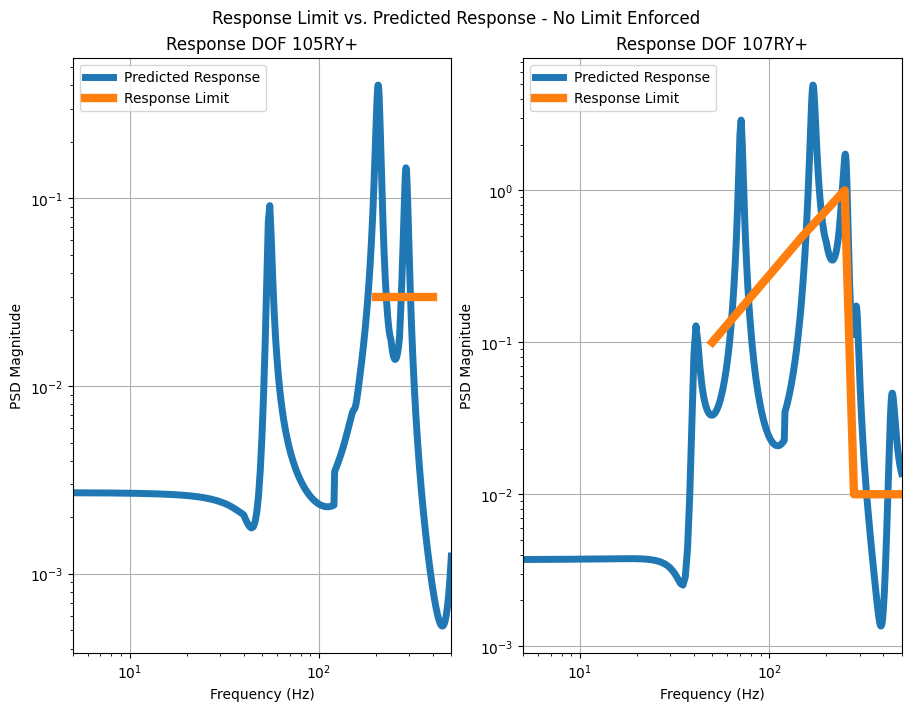
The predicted responses (from the estimated drives without the limits enforced) are also compared to the response limits, showing that there are several frequencies where the limits are exceeded.

Note

The predicted responses are compared to the limits on log-log plots since that is how limits are commonly specified in vibration testing.

fig, ax = plt.subplots(1,2, layout='constrained', figsize=(9,7))
fig.suptitle('Response Limit vs. Predicted Response - No Limit Enforced')

ax[0].loglog(no_limit_spr.abscissa, 
    np.abs(no_limit_spr.predicted_response_specific_dofs(example_limit[0].limit_coordinate).ordinate[0,0,:]),
    label='Predicted Response', linewidth=5)
ax[0].loglog(example_limit[0].breakpoint_frequency, example_limit[0].breakpoint_level, 
             label='Response Limit', linewidth=6)
ax[0].grid()
ax[0].legend()
ax[0].set_xlabel('Frequency (Hz)')
ax[0].set_ylabel('PSD Magnitude')
ax[0].set_xlim(left=5, right=500)
ax[0].set_title('Response DOF '+example_limit[0].limit_coordinate.string_array()[0]);

ax[1].loglog(no_limit_spr.abscissa, 
    np.abs(no_limit_spr.predicted_response_specific_dofs(example_limit[1].limit_coordinate).ordinate[0,0,:]),
    label='Predicted Response', linewidth=5)
ax[1].loglog(example_limit[1].breakpoint_frequency, example_limit[1].breakpoint_level, 
             label='Response Limit', linewidth=6)
ax[1].grid()
ax[1].legend()
ax[1].set_xlabel('Frequency (Hz)')
ax[1].set_ylabel('PSD Magnitude')
ax[1].set_xlim(left=5, right=500)
ax[1].set_title('Response DOF '+example_limit[1].limit_coordinate.string_array()[0]);

Applying the Limits

The response limits are applied by supplying the example_limit object to the apply_response_limit method for the PowerSourcePathReceiver. There are three important options for the apply_response_limit method:

1. limit_db_level: This option determines if the limit should be adjusted by the supplied dB level. This is important for cases where the limits were developed for a specific test level that is different from what is being used. For example, the limit may have been developed for a “qualification” level whereas the test is being ran at a “workmanship” (e.g., -6 dB) level.

2. interpolation_type: This option determines how the limit breakpoints will be interpolated to the abscissa for the SPR object. Essentially, this determines if the lines between breakpoints should be straight on a linear-linear or log-log plot.

3. in_place: This determines if the apply_response_limit method should save the modified drives to the original SPR object or if it should return a new SPR object with the original object unchanged.

limit_spr = no_limit_spr.apply_response_limit(example_limit, 
                                              limit_db_level=0,
                                              interpolation_type='loglog', 
                                              in_place=False)

It is generally good practice to evaluate how scaling the drives to enforce the response limit effects the accuracy of the test. This is done below with the error_summary method. These plots show that enforcing the response limits will effect all the response DOFs in the source estimation problem, potentially causing significant errors in the frequency bands where the predicted response exceeded the limit.

limit_spr.error_summary(figure_kwargs={'figsize':(9,7)}, linewidth=5)

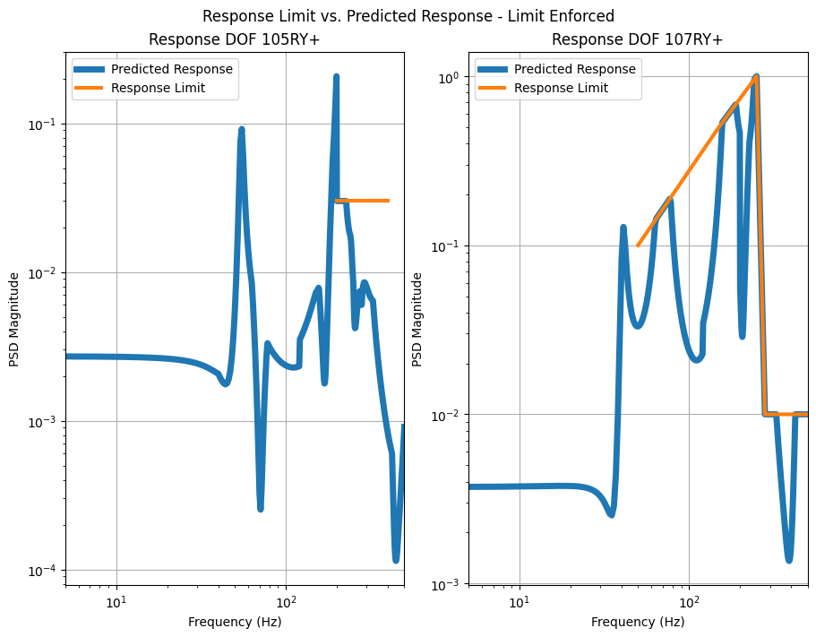
The predicted responses from the drives with the limits enforced show that the updated prediction is compliant with the limits. This plot also shows how a limit on one DOF can supersede the limit on another DOF, since the 300 Hz peak in 105RY+ is dramatically reduced by the limit that is applied to 107RY+.

fig, ax = plt.subplots(1,2, layout='constrained', figsize=(9,7))
fig.suptitle('Response Limit vs. Predicted Response - Limit Enforced')

ax[0].loglog(limit_spr.abscissa, 
    np.abs(limit_spr.predicted_response_specific_dofs(example_limit[0].limit_coordinate).ordinate[0,0,:]),
    label='Predicted Response', linewidth=5)
ax[0].loglog(example_limit[0].breakpoint_frequency, example_limit[0].breakpoint_level, 
             label='Response Limit', linewidth=3)
ax[0].grid()
ax[0].legend()
ax[0].set_xlabel('Frequency (Hz)')
ax[0].set_ylabel('PSD Magnitude')
ax[0].set_xlim(left=5, right=500)
ax[0].set_title('Response DOF '+example_limit[0].limit_coordinate.string_array()[0]);

ax[1].loglog(limit_spr.abscissa, 
    np.abs(limit_spr.predicted_response_specific_dofs(example_limit[1].limit_coordinate).ordinate[0,0,:]),
    label='Predicted Response', linewidth=5)
ax[1].loglog(example_limit[1].breakpoint_frequency, example_limit[1].breakpoint_level, 
             label='Response Limit', linewidth=3)
ax[1].grid()
ax[1].legend()
ax[1].set_xlabel('Frequency (Hz)')
ax[1].set_ylabel('PSD Magnitude')
ax[1].set_xlim(left=5, right=500)
ax[1].set_title('Response DOF '+example_limit[1].limit_coordinate.string_array()[0]);