Inverse Problem Form#
All the SPR types in ForceFinder solve the ISE problems using FRF matrix inversion, with different implementations depending on the response type. Refer to the SPR Types section to recall the different response types. Consequently, the problem form is based on the FRF equation of motion for the system with a particular response type. The LinearSourcePathReceiver uses the most basic problem form, where responses are computed with:
The accompanying pseudo-inverse ISE method for the LinearSourcePathReceiver is:
This problem form is easily converted for CPSDs via the following operation:
As such, the forward prediction for the PowerSourcePathReceiver is:
The accompanying pseudo-inverse ISE method for the PowerSourcePathReceiver is:
Note
This section only shows the most basic inverse method. Other, more complex inverse methods will be described elsewhere.
FRF Inverse with the Singular Value Decomposition#
Many of the inverse methods in ForceFinder compute the pseudo-inverse of the FRF matrix via its singular value decomposition:
Where the pseudo-inverse is:
While the distinction in how the pseudo-inverse is calculated is not important for the pseudo-inverse method, it is useful to understand for other methods like Tikhonov regularization or the truncated singular value decomposition (TSVD).
Note
Many methods invert the matrix of singular values via element-wise division (since it is a diagonal matrix). Some methods may need to compute an actual inverse if off-diagonal terms are added to the singular value matrix.
COLA Method for Transient Inverse Problems#
The TransientSourcePathReceiver uses the same inverse problem form as the LinearSourcePathReceiver, except additional pre and post processing is required to handle the deconvolution aspects of the time domain source estimation. This pre and post processing is handled in the transient_inverse_processing decorator function. An abridged description of the process is:
The full response time trace is zero padded to avoid any spoilage from the windowing in the COLA procedure.
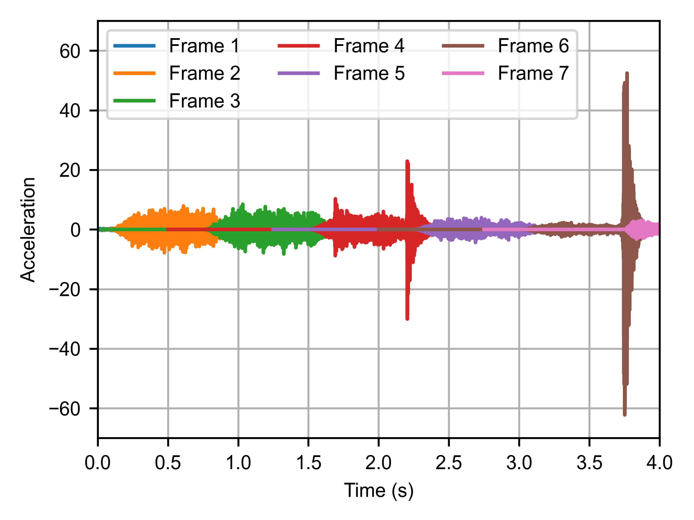
The response time trace (from step one) is split into overlapped and windowed segments. The default segment block time is set to match the frequency resolution of the FRFs and the default window is a Tukey with an alpha parameter of 0.5, which uses a 25% overlap for a COLA condition. These parameters can be changed from the defaults by supplying optional kwargs when calling the inverse method. An example of this segmentation is shown in in the figure below.
The segmented time responses (from step two) are zero padded to avoid any convolution wraparound errors.
The windowed, segmented, and zero padded time responses (from step three) are converted to the frequency domain with a discrete Fourier transform (DFT).
The FRFs are interpolated to match the frequency resolution of the frequency domain responses from step four.
The frequency domain response (from step four) and interpolated FRFs (from step five) are used to estimate the sources with the same inverse problem form as the
LinearSourcePathReceiver.The frequency domain sources (for each time segment) are converted to the time domain using an inverse DFT.
The segmented time domain sources are recompiled into a single time trace for the whole time.
Warning
While the sources for the TransientSourcePathReceiver are estimated in the frequency domain, it is still a deconvolution process where the FRFs can be viewed as finite impulse response (FIR) filters. As such, the practitioner must be careful to avoid issues related to non-causal filtering.
The most significant of these issues are apparent non-causalities in the FRFs. There are not any techniques in ForceFinder to mitigate these apparent non-causalities, but the enforce_causality method in SDynPy is suggested to pre-process the FRFs before SPR object initialization.
Note
It may be useful to review the inverse method code layout for the TransientSourcePathReceiver to reinforce how the COLA method works in the ISE problem.
Reason for Using the COLA method#
The COLA procedure is used in ForceFinder instead of pure deconvolution, adaptive filtering, or modal methods for the following reasons:
The COLA procedure uses the same force estimation methods as linear spectra, which has been widely researched. Further, this problem form is the same as the supervised learning approach for machine learning, where there has been a dramatic amount of research on inverse problems.
Pure deconvolution can be extremely computationally inefficient, especially for long time responses.
The COLA procedure directly uses FRFs, which eliminates the need for additional assumptions and data processing to develop a modal description of the system (when the FRF data is based on experiments).