Implementation

In this section, the implementation of the WEC Module within the SNL-SWAN code will be described in detail. This section explains how the WEC Module was formulated from the SWAN (Version 41.20) code.

SNL-SWAN models WEC devices as obstacles using the five “obcase” flags listed below to determine the appropriate obstacle transmission coefficient. The following section describes the SNL-SWAN treatment of WEC devices under each obstacle case model.

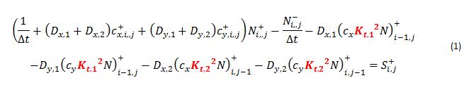
Section 3.10 of the SWAN Scientific and Technical Documentation describes the effect of obstacles through a coefficient in the convection terms of the action density evolution equation. The action density equation is shown below Eq.(1) with the obstacle transmission coefficient boxed in red. The sole difference between the obstacle cases is the method of obtaining this value. The five methods are described below. A visual conceptual comparison is shown at the end of this section.

OBCASE 0

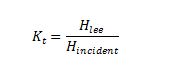
This is the standard, TUDelft SWAN, obstacle treatment. The value K_t is a constant value entered into the SWAN input file. K_t represents the ratio of wave heights incident to and lee of the obstacle (or WEC).

OBCASE 1

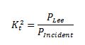
Obstacle case 1 uses the WEC power matrix to calculate the effective transmission coefficient. In this case, K_t^2 is calculated using the provided power matrix, and a constant value for this coefficient is used across all frequencies. K_t^2 represents the energy (or power) ratio incident and lee of the obstacle.

The power matrix is a table of absorbed power (in Kilowatts, kW) by a WEC device over varying significant wave heights and peak wave periods. SNL-SWAN determines the incident significant wave height and the incident peak wave period and then linearly interpolates a value for absorbed power from the matrix. Note: if the incident values for wave height or period lie outside of the power matrix range, a value of zero is returned.

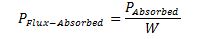
The absorbed power flux (power per unit width) of the obstacle is determined by dividing the interpolated value for absorbed power by the “width” value provided as the first entry in the Power.txt file. Note that the width value here should be thought of as a normalization value, and is only used to convert the power matrix entries of absorbed power (kW) into absorbed flux (kW/m) values. This value is calculated as follows.

This value is then applied evenly across the entire obstacle, as defined in the main INPUT file. In most cases the width value in Power.txt should be the same as the length of the obstacle defined in the INPUT file, but this is not required by the model. There are no checks in the code to guarantee or enforce this equality.

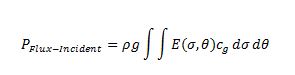
SNL-SWAN then calculates the incident power fluxing across the obstacle (in kW/m). The power fluxing over the obstacle is calculated directly from the spectral information incident to the obstacle.

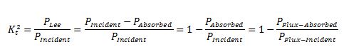
To determine the transmission coefficient, SWAN takes the incident power flux and subtracts off absorbed power flux. The transmission coefficient is the ratio of the remaining flux to the incident flux, and K_t^2 is calculated using the following equation:

When the action balance equation is solved, the convection term, N(s,theta)c_g K_t^2, will be applied (integrated) across the computational width of the obstacle. The computational width (as opposed to the width defined in the power matrix file) is determined by the obstacle dimensions defined in the main SWAN INPUT file and the grid discretization (See the section on Grid Treatment).

OBCASE 2

Obstacle case 2 uses the WEC relative capture width curve to calculate the effective transmission coefficient. K_t^2 is again calculated using the provided curve, and a constant value is used across all frequencies.

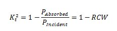
The relative capture width curve is a table of absorbed power ratios by a WEC device at varying wave periods. In ways, this implementation is simpler than that or the power matrix. Since the relative capture width curve already provides power ratios, K_t^2 is more straightforward to calculate without the need to determine the incident power flux. For this case, SNL-SWAN linearly interpolates an RCW value from the curve given the peak incident wave period, and directly calculates a transmission coefficient using the following relation. As with obstacle case 1, any wave periods outside of the defined range are given a transmission coefficient of zero.

OBCASE 3

SNL-SWAN’s obstacle case 3 is just an extension of case 1. This case behaves exactly the same way as case 1, except that the routine to determine the transmission coefficient is performed separately for each binned frequency of the model. This in effect makes K_t^2 a function of frequency, resulting in varying power absorption for waves of different frequency. Note: while the power matrix is defined in terms of wave period, internal SWAN calculations are all performed using wave frequency. Each computational frequency is converted to a wave period as follows before interpolating from the power matrix.

OBCASE 4

SNL-SWAN’s obstacle case 4 is an extension of case 2. Again, the only difference is that the RCW curve is sampled independently for each frequency of the simulation, resulting in a frequency dependent obstacle transmission coefficient.

OBCASE 5

Note

This section is under development

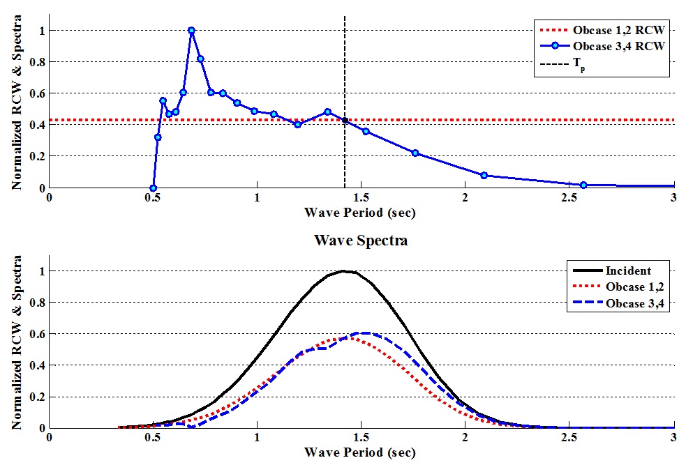
OBCASE Comparison

Differences between SNL-SWAN OBCASE options are visualized in Figure XX. In this figure a conceptual frequency independent RCW curve which would be the case for OBCASE 1 and 2 is shown as the dotted red line in the top panel. The frequency dependent OBCASES 3 and 4 would have a RCW curve that is variable dependent on frequency, as indicated by the blue line in the top panel. The resultant wave spectra in the lee of the obstacle for these cases are shown in the bottom panel, as compared to the incident spectra (black line).