Best Practices

In this section SNL-SWAN best practices are given for the use of the SNL-SWAN to model WECs. This section is meant to address frequently addressed questions.

Grid Treatment

As noted in Section 3.10 of the SWAN Scientific and Technical Documentation, obstacles are treated as lines running through the computational grid. When calculating the action density flux from one grid point to its neighbors, SWAN first determines if the connecting grid line crosses an obstacle line. If and only if a grid line is crossed by an obstacle line, the transmission coefficient applied to the flux between those nodes.

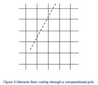
As described in Section 5.2.1 of the SWAN Scientific and Technical Documentation, SWAN uses a vertex centered grid, with volume cells defined by grid centers. Figure 4 below shows a computational grid (solid lines), a grid vertex, and the finite volume cell corresponding to that vertex (dashed lines). The finite volume cell edges are the fluxing faces between neighboring vertices.

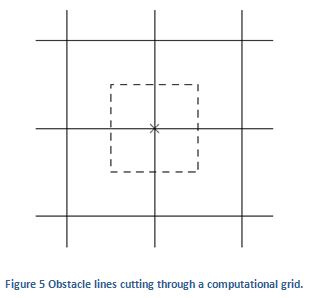
This grid treatment in combination with SWAN’s obstacle treatment has some implications which should be noted. Figure 5 shows the various ways in which obstacles can interact with the computational grid.

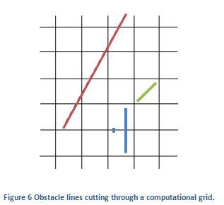
The two blue obstacles shown in Figure 5 will have the exact same influence on the model solution, even though they have much different widths. Since both obstacles cross the same computation grid line, SWAN will apply their transmission coefficient the same volumetric fluxing face. The straight dashed lines in Figure 4 show the fluxing faces of a cell volume. Both obstacles correspond to the same face, and thus their obstacle coefficients will have the same impact on the model calculation.

Due to grid discretization, the green obstacle in Figure 5 does not intersect and computational grid lines. In this situation it will have no effect, even though the obstacle is much larger than the small blue obstacle (which does have an effect).

The red line in Figure 5 shows the appropriate use of the obstacle implementation, where grid discretization is much finer than the obstacle length. This means that obstacles will span multiple grid lines and their length and transmission effects can be properly captured.

WEC Power Performance

It should be noted that RCW values should be kept between zero and one (0<RCW<1) in order to produce physical transmission coefficients. Should RCW values be specified outside of these bounds, SNL-SWAN will enforce these limits in order to maintain realizable values for the transmission coefficient.

In choosing an obstacle case, attention should be paid to the way the Power Matrix or RCW curve was created. Using OBCASE equal to 3 or 4 is only appropriate when information is available about individual frequencies. OBCASE 1 and 2 are more appropriate when information is available about average sea states. Power Matrices may be populated with information derived from either regular waves, or irregular real sea waves. When working with a Power Matrix populated with regular waves, it makes sense to use OBCASE=3. However, when working with a Power Matrix which has been populated using values aggregated over real sea waves, it is more appropriate to use OBCASE=1.

Transmission coefficients are obtained through interpolation between points in either the Power Matrix or the RCW curve. Any frequency or significant wave height lying outside the bounds specified in these files will be given a transmission coefficient of 1.0 (an absorption coefficient of 0.0). SNL-SWAN will not extrapolate values outside of these ranges, and the user is encouraged to modify their input curves should they desire this behavior.