ufjc.swfjc

The core module for the SWFJC single-chain model.

This module contains the core class SWFJC which, upon instantiation, becomes a SWFJC single-chain model instance with methods for computing single-chain quantities in either thermodynamic ensemble. The SWFJCIsometric and SWFJCIsotensional classes are also contained within this module. The SWFJC is the uFJC model with a square-well link potential, which is a special case that is efficiently treated separately as it can be solved exactly [1].

Example

Import and create an instance of the model:

>>> from ufjc import SWFJC
>>> model = SWFJC()

class SWFJC

Bases: SWFJCIsotensional

The SWFJC single-chain model class.

N

The number of links in the chain.

Type:

int

varsigma

The nondimensional well width.

Type:

float

class SWFJCIsometric(N_b=8, varsigma=3)

Bases: BasicUtility

The SWFJC model class for the isometric ensemble.

N

The number of links in the chain.

Type:

int

varsigma

The nondimensional well width.

Type:

float

class SWFJCIsotensional(N_b=8, varsigma=2)

Bases: SWFJCIsometric

The SWFJC model class for the isotensional ensemble.

N

The number of links in the chain.

Type:

int

varsigma

The nondimensional well width.

Type:

float

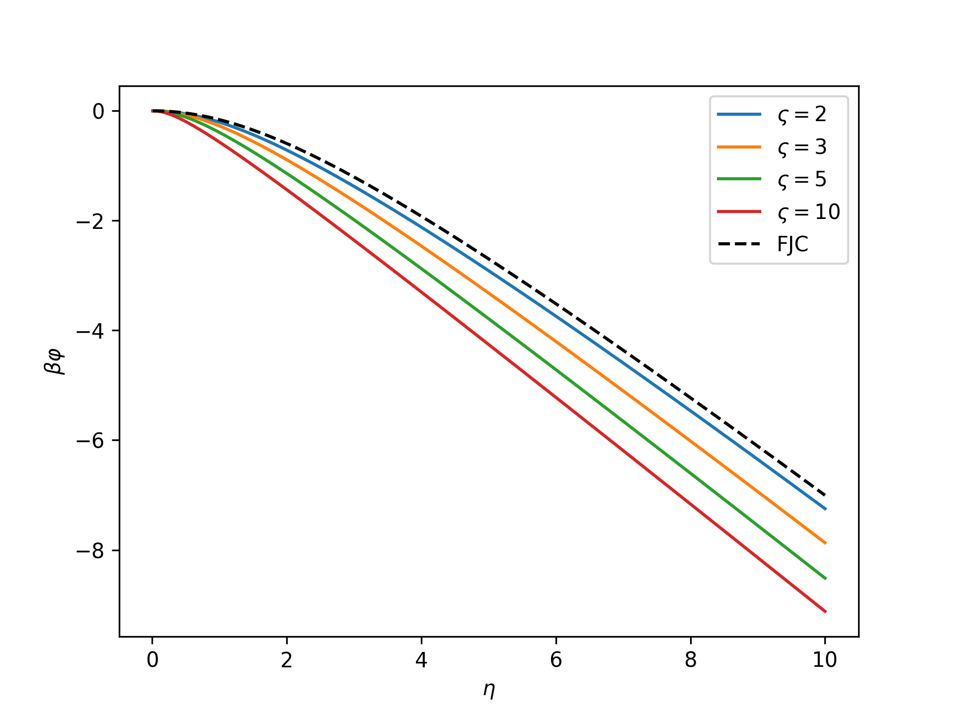
beta_varphi(eta)

The nondimensional isotensional free energy as a function of the nondimensional force,

$$\beta \phi (\eta )=-\ln \mathfrak{z}(\eta ).$$

Note that this becomes the isotensional free energy of the FJC model as $\varsigma$ goes to zero,

$$\underset{\varsigma \to 0}{lim}\beta \phi (\eta )=\ln \left[\frac{\eta }{\sinh (\eta )}\right].$$

Parameters:

v (array_like) – The nondimensional force.

Returns:

The nondimensional isotensional free energy.

Return type:

numpy.ndarray

Example

Plot the nondimensional isotensional free energy as a function of the nondimensional force for varying $\varsigma$:

>>> import numpy as np
>>> import matplotlib.pyplot as plt
>>> from ufjc.swfjc import SWFJCIsotensional
>>> eta = np.linspace(0, 10, 1000)[1:]
>>> _ = plt.figure()
>>> for varsigma in [2, 3, 5, 10]:
...     model = SWFJCIsotensional(varsigma=varsigma)
...     _ = plt.plot(eta, model.beta_varphi(eta),
...                  label=r'$\varsigma=$'+str(varsigma))
>>> _ = plt.plot(eta, np.log(eta/np.sinh(eta)),
...              'k--', label='FJC')
>>> _ = plt.xlabel(r'$\eta$')
>>> _ = plt.ylabel(r'$\beta\varphi$')
>>> _ = plt.legend()
>>> plt.show()

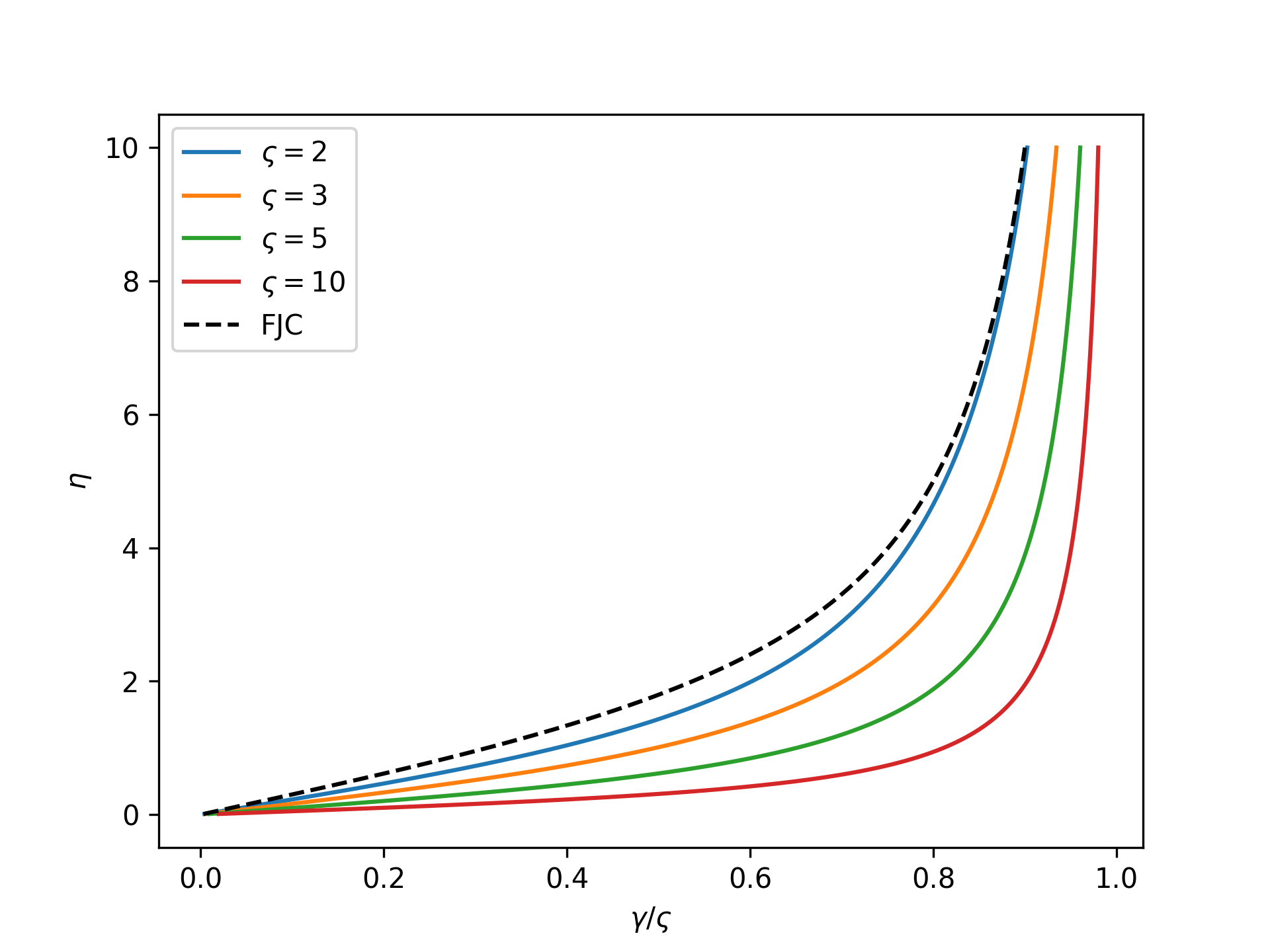
gamma_isotensional(eta)

The nondimensional end-to-end length as a function of the nondimensional force in the isotensional ensemble,

$$\gamma (\eta )=\frac{\partial }{\partial \eta }\ln \mathfrak{z}(\eta )=\frac{{\varsigma }^2\eta \sinh (\varsigma \eta )-\eta \sinh (\eta )}{\varsigma \eta \cosh (\varsigma \eta )-\sinh (\varsigma \eta )-\eta \cosh (\eta )+\sinh (\eta )}$$

Note that this becomes the Langevin function of the FJC model as $\varsigma$ goes to zero,

$$\underset{\varsigma \to 0}{lim}\gamma (\eta )=\coth (\eta )-\frac{1}{\eta }=\mathcal{L}(\eta ).$$

Parameters:

v (array_like) – The nondimensional force.

Returns:

The nondimensional end-to-end length.

Return type:

numpy.ndarray

Example

Plot the nondimensional single-chain mechanical response in the isotensional ensemble for varying $\varsigma$:

>>> import numpy as np
>>> import matplotlib.pyplot as plt
>>> from ufjc.swfjc import SWFJCIsotensional
>>> eta = np.linspace(0, 10, 1000)[1:]
>>> _ = plt.figure()
>>> for varsigma in [2, 3, 5, 10]:
...     model = SWFJCIsotensional(varsigma=varsigma)
...     _ = plt.plot(
...         model.gamma_isotensional(eta)/varsigma,
...         eta, label=r'$\varsigma=$'+str(varsigma))
>>> _ = plt.plot(1/np.tanh(eta) - 1/eta, eta,
...              'k--', label='FJC')
>>> _ = plt.xlabel(r'$\gamma/\varsigma$')
>>> _ = plt.ylabel(r'$\eta$')
>>> _ = plt.legend()
>>> plt.show()

z(eta)

The nondimensional single-link isotensional partition function as a function of the nondimensional force,

$$\mathfrak{z}(\eta )=\frac{1}{{\eta }^3}[\varsigma \eta \cosh (\varsigma \eta )-\sinh (\varsigma \eta )-\eta \cosh (\eta )+\sinh (\eta )].$$

Parameters:

v (array_like) – The nondimensional force.

Returns:

The nondimensional isotensional partition function.

Return type:

numpy.ndarray

---

References

[1]

Michael R. Buche, Meredith N. Silberstein, and Scott J. Grutzik. Freely jointed chain models with extensible links. Physical Review E, 106(024502):024502, 2022. doi:10.1103/PhysRevE.106.024502.