Tutorial

This is a tutorial demonstrating the basics of the Python package ufjc.

Model Creation

The uFJC single-chain model is imported from the package as the uFJC class,

>>> from ufjc import uFJC

Instantiating the class creates a particular model instance,

>>> model = uFJC()

Keyword arguments allow model features to be selected during instantiation, such as choosing 8 links and a nondimensional link energy scale of 88:

>>> model = uFJC(N_b=8, varepsilon=88)

Keyword arguments also provide a way to change the link potential energy function and associated parameters, i.e.

>>> model = uFJC(potential='morse', N_b=8, varepsilon=88, alpha=1)

Model Functions

The model instance has many single-chain functions attributed, such as gamma, the nondimensional single-chain mechanical response function,

>>> model.gamma
<bound method uFJC.gamma of <ufjc.core.uFJC object at 0x7f2ca1b53160>>

This function takes the nondimensional force eta as an argument, as well as keyword arguments. For example,

>>> model.gamma(0.55)
array([0.18780929])

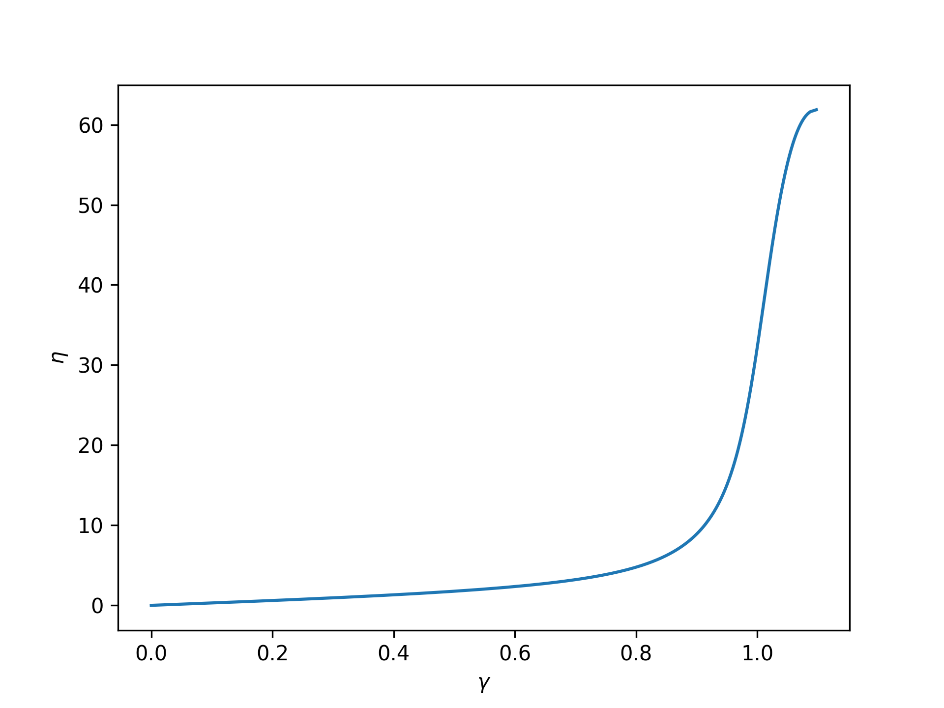
An array of nondimensional forces can be input, and these results can be easily plotted:

>>> import numpy as np
>>> import matplotlib.pyplot as plt
>>> from ufjc import uFJC
>>> model = uFJC(potential='lennard-jones', varepsilon=23)
>>> eta = np.linspace(0, model.eta_max, 250)
>>> plt.plot(model.gamma(eta), eta)
>>> plt.xlabel(r'$\gamma$')
>>> plt.ylabel(r'$\eta$')
>>> plt.show()

Thermodynamic Ensembles

Generally, the results differ whether a constant force or a constant end-to-end length is applied to the chain. These are the isotensional and isometric ensembles, respectively, also sometimes called the Gibbs and Helmholtz ensembles. Here, the method refers to the method of calculating results in the isometric ensemble. For example, we can use the legendre approximation method to compute eta in the isometric ensemble at a nondimensional end-to-end length of 0.23,

>>> model.eta(0.23, ensemble='isometric', method='legendre')
array([0.70164801])

Calculation Approaches

For the isotensional ensemble, there are several calculation approaches available: exact closed-form (FJC, EFJC), numerical quadrature, Monte Carlo, and asymptotically-correct approximations. Here, the approach refers to the calculation approach for results in the isotensional ensemble. For example, we can use the reduced asymptotic approach to compute gamma in the isotensional ensemble (default) under a nondimensional force of 55,

>>> model.gamma(55, approach='reduced')
array([1.0441542])

Combinations

Since neither ensemble is typically exactly analytically tractable, we often need to combine approximations methods and approaches when working with the isometric ensemble. The above example for the isometric ensemble actually used the asymptotic approach, since it is the default,

>>> model.eta(0.23, ensemble='isometric', method='legendre', approach='asymptotic')
array([0.70164801])

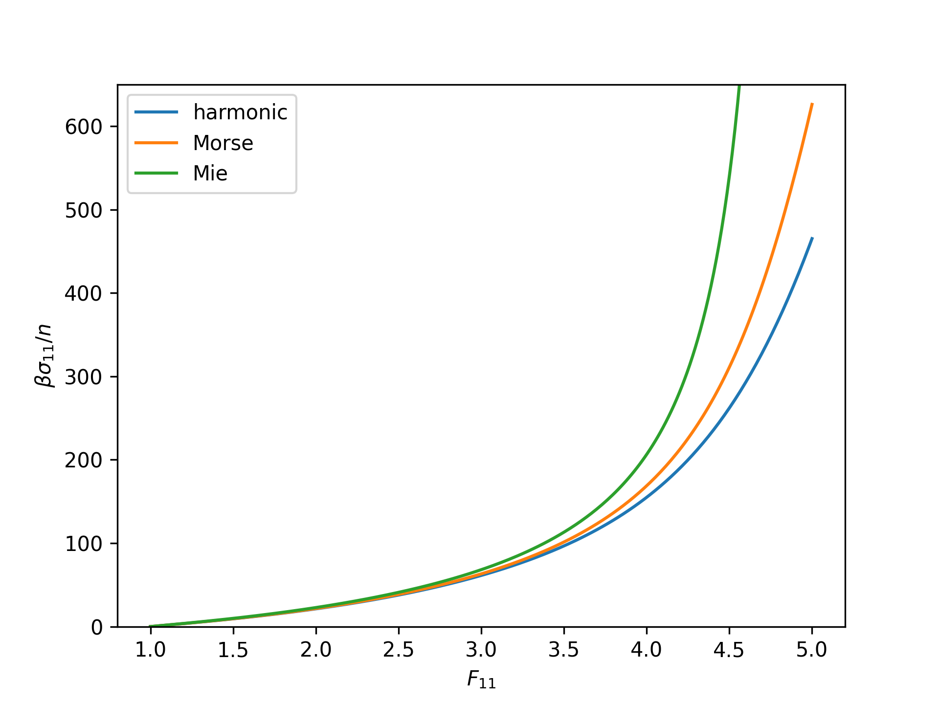
Outside Applications

Model is readily applicable outside the scope of this package, such as to network constitutive models. Here, we apply a few different uFJC models to the eight-chain model configuration:

>>> import numpy as np
>>> import matplotlib.pyplot as plt
>>> from ufjc import uFJC
>>> def beta_sigma_11(F_11, **kwargs):
...     model = uFJC(**kwargs)
...     I_1 = F_11**2 + 2/F_11
...     lambda_chain = np.sqrt(I_1/3)
...     gamma = lambda_chain/np.sqrt(model.N_b)
...     eta = model.eta(gamma)
...     return model.N_b*eta/lambda_chain*(F_11**2 - I_1/3)
>>> F_11 = np.linspace(1, 5, 250)
>>> beta_sigma_11_harmonic = beta_sigma_11(F_11, N_b=8)
>>> beta_sigma_11_morse = beta_sigma_11(F_11, potential='morse', N_b=8)
>>> beta_sigma_11_mie = beta_sigma_11(F_11, potential='mie', N_b=8)
>>> plt.plot(F_11, beta_sigma_11_harmonic)
>>> plt.plot(F_11, beta_sigma_11_morse)
>>> plt.plot(F_11, beta_sigma_11_mie)
>>> plt.legend(['harmonic', 'Morse', 'Mie'])
>>> plt.xlabel(r'$F_{11}$')
>>> plt.ylabel(r'$\beta\sigma_{11}/n$')
>>> plt.ylim(0, 650)
>>> plt.show()