E2Synthetic Example Problem with a SDynPy System
This example problem will utilize the Python package SDynPy[1] to construct a System object that can be integrated over time to produce a synthetic control problem in Rattlesnake. This example problem can run entirely on a desktop or laptop computer and does not require any dedicated data acquisition, instrumentation, or shaker hardware. Synthetic tests are therefore very useful for developing an understanding of how Rattlesnake works. Rattlesnake deliberately tries to make its synthetic operation look as close as possible to running a real test, which makes it useful for learning or trying out new things without worrying about breaking an expensive piece of equipment if a mistake is made. For more information in using SDynPy objects with Rattlesnake, see Chapter 10.
This test problem will largely mirror the example problem from Example E1, but will be performed synthetically.
The general process for this control problem is as follows:
Import the SDynPy package.
Create a
Systemobject for the structure, consisting of a Mass, Stiffness, and Damping matrix.Select degrees of freedom to control
Create a specification to make Rattlesnake try to achieve
Create Rattlesnake tests for MIMO Random Vibration, MIMO Transient, and Modal Testing environments.
Load the Rattlesnake data back into SDynPy to make comparison plots.
Being a Python package, we run SDynPy from within a Python environment. The author is using Python 3.11 for this example. The full source code for this example is attached to this document as a .txt file[2], which can be transformed to a Python file by renaming the .txt to .py.
2.1Creating a SDynPy System and Specifications for Random and Transient Vibration Tests
This section will contain the SDynPy commands that will be used to set up the test.
2.1.1Importing Relevant Python Packages
In order to use SDynPy and other Python Packages, they need to be imported
# Import SDynPy module to get structural dynamics functionality
import sdynpy as sdpy
# We'll also import some common Python packages
import numpy as np # NumPy for numeric calculations
import matplotlib.pyplot as plt # Matplotlib for plotting2.1.2Creating the Demonstration Objects
Next we will construct the demonstration objects. We will construct Geometry and System objects from a beam finite element model that we create with SDynPy. The Geometry contains all of the spatial information about the object: locations and orientations of various degrees of freedom on the structure, as well as connections between them. The System contains the dynamic information: mass, stiffness, and damping matrices and the degrees of freedom associated with each row and column of those matrices.
We will plot the degrees of freedom on the geometry to help us understand where we would like to perform measurements and place excitation devices. The results are shown in Figure E2.1.
# Create a system and geometry object using the beam functionality in SDynPy
system,geometry = sdpy.System.beam(
    length = 24 * 0.0254, # meters
    width = 0.75 * 0.0254, # meters
    height = 1.0 * 0.0254, # meters
    num_nodes = 25,
    material = 'steel')
# We want to see which degrees of freedom we have to work with, so we will
# plot the geometry with coordinate labels
geometry.plot_coordinate(label_dofs=True,arrow_scale=0.02)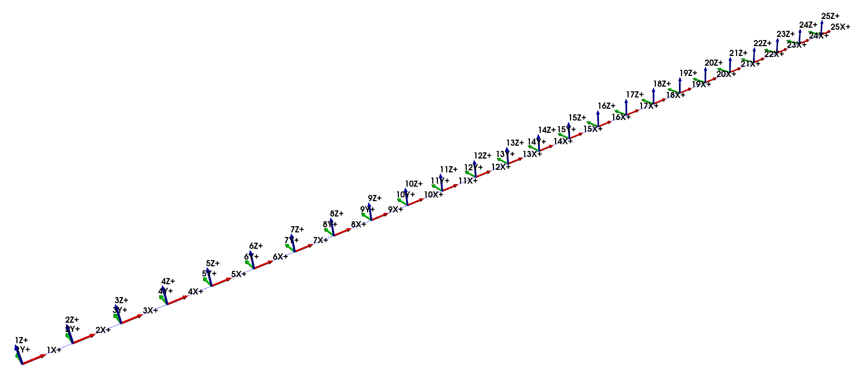
Figure E2.1:Geometry and degrees of freedom from the beam finite element model.
Because Rattlesnake will try to integrate equations of motion real-time, it is useful if we can get a reduced-order model of the structure to integrate. Transforming to a modal model is a natural choice, as it will reduce the number of degrees of freedom as well as uncouple them. It also affords us the ability to add modal damping to the structure, which can make the test more realistic. SDynPy will keep track of the modal transformation (mode shape matrix) that transforms the modal degrees of freedom back to physical degrees of freedom.
# The finite element model system of equations is too large to integrate
# real-time, so we will create a reduced modal system to integrate based on the
# desired bandwidth of the test
test_bandwidth = 2560 # Hz

# Solve for modes up to 1.5x the bandwidth to lessen modal truncation effects
modes = system.eigensolution(maximum_frequency = test_bandwidth*1.5)

# This also gives us the option to add some damping to the model
modes.damping = 0.005

# Transform to modal system: modal mass, modal stiffness, modal damping
modal_system = modes.system()

# Save it to a file that we will load in Rattlesnake
modal_system.save('sdynpy_system.npz')2.1.3Selecting Degrees of Freedom
We will now select the degrees of freedom for this test. We will compute a vibration specification at these degrees of freedom that we will later use to control the test. In this case, we will select the same response degrees of freedom as from Example E1. Note, however, that the node numbers will be offset by 1 from that test, as the node that is 1 inch from the end of the beam is actually called node 2 in our finite element model. Figure E2.2 shows these degrees of freedom.
We will also select some excitation degrees of freedom that we will use to hit repeatedly with a hammer impact, similar to what was done in Section 1.3.1 to create the vibration specification. We will integrate equations of motion where the excitation is random strikes at each of these nodes in the same way we measured the response to random tapping on the beam in the real test. Note that these are not the nodes where shakers will be placed in the actual modal and vibration tests, but are only used to construct the specification. Figure E2.3 shows these degrees of freedom.
# Now let's select some degrees of freedom for our test.  We will measure all
# points in the vertical (z) direction.
response_dofs = sdpy.coordinate_array([2,13,19,24],'Y-')

# Let's also select some excitation degrees of freedom for the test
excitation_dofs = sdpy.coordinate_array(geometry.node.id[::3],'Y-')

geometry.plot_coordinate(response_dofs,label_dofs=True,arrow_scale=0.05)
geometry.plot_coordinate(excitation_dofs,label_dofs=True,arrow_scale=0.05)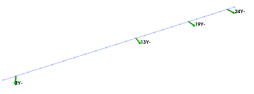
Figure E2.2:Degrees of freedom measured and used to control the vibration test.
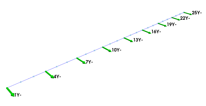
Figure E2.3:Degrees of freedom at which random hammer impacts will be applied to construct a vibration environment.
2.1.4Simulating an Environment
With the system set up and degrees of freedom selected, we will now integrate the equations of motion to generate specifications that we can use to control the test. We will apply a multi-hammer impact to each of the nodes in Figure E2.3 and extract responses at the nodes in Figure E2.2.
# Let's simulate the multi-hammer impact that was performed on the test article
# in the example problem

frame_length = test_bandwidth*2 # Samples

responses, references = modal_system.simulate_test(
    bandwidth = test_bandwidth,
    frame_length = frame_length,
    num_averages = 30,
    excitation = 'multi-hammer',
    references = excitation_dofs,
    responses = response_dofs,
    excitation_level = 0.1,
    excitation_max_frequency = test_bandwidth*1.5)
This will give us 30 averages of the multi-hammer excitation that we will use to construct specifications. From the response data we will construct a CPSD matrix. The APSDs are shown in Figure E2.4.
# Now we will convert that into a CPSD and a transient specification that we
# will try to replicate.
cpsd = responses.cpsd(frame_length, overlap = 0.0, window = 'boxcar')

# We'll truncate the low frequency to make sure that we don't get huge rigid
# body response as well as the high frequency above the antialiasing filters of
# the system
cpsd.ordinate[(cpsd.abscissa < 20) | (cpsd.abscissa > 2000)] = 0

# Plot the diagonal so we can see levels
cpsd.plot_asds({'layout':'constrained','sharex':True,'sharey':True})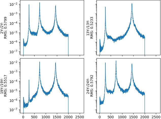
Figure E2.4:Specification for the MIMO Random Vibration test.
We will also pull off the first frame of data to use as a specification for a transient test, shown in Figure E2.5.
# We'll also grab just the first average to make into a rattlesnake transient
# specification
transient = responses.idx_by_el[:frame_length]

transient.plot(
    one_axis=False,
    subplots_kwargs={'layout':'constrained'},
    plot_kwargs={'linewidth':0.5})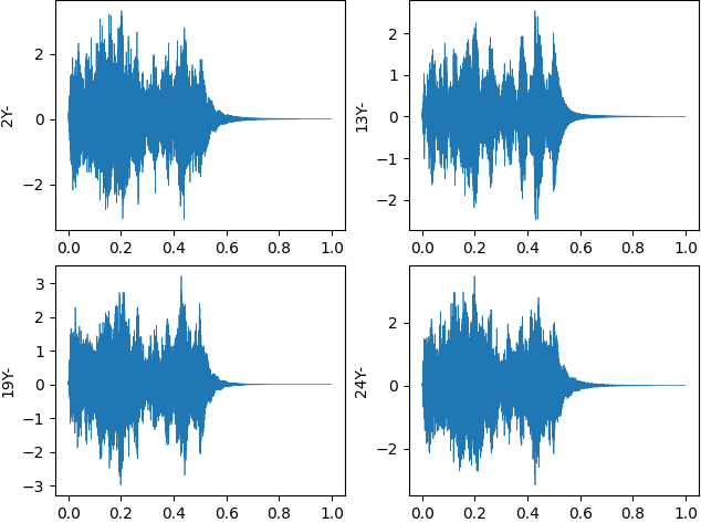
Figure E2.5:Specification for the MIMO Transient Vibration test.
We can then save these files to disk.
# Now we can save these to specifications for Rattlesnake
cpsd.to_rattlesnake_specification('random_specification.npz')
transient.to_rattlesnake_specification('transient_specification.npz')2.2Running a Synthetic Modal Test
Now that we have the pieces of information required, we can run our modal and vibration tests. The primary difference between this test and the one run in Example E1 is that there is no voltage signal being measured, only forces. The SDynPy object we will be integrating does not know anything about any shaker we might attach to the structure, it only knows about the test article’s dynamics. This means “inputs” to the system are forces rather than voltages.
Another major difference between this test and the previous on from Example E1 is that it is more difficult to perform a synthetic hammer impact test. One can achieve this by using the combined environments capabilities of Rattlesnake, specifying perhaps a Time History Generator environment to provide a impact-like pulse, which could be used to trigger the modal acquisition. However, this advanced usage is out of the scope of this beginner-level tutorial, so it will not be discussed here.
2.2.1Data Acquisition Setup
Similarly to Example E1, we will open Rattlesnake in the Modal Environment to save out a channel table template that we will use for this test. Rather than filling out the channel table in the GUI, we will load it from an Excel spreadsheet, which allows us to more easily save our work. We can get a template channel table to fill out by opening Rattlesnake and selecting the Modal Testing environment (Figure E2.6).
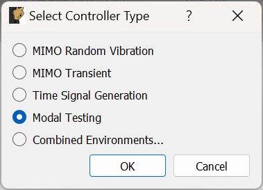
Figure E2.6:Selecting the Modal Environment in Rattlesnake
We can then click the Save Channel Table button to save out the empty channel table to an Excel spreadsheet (Figure E2.7).
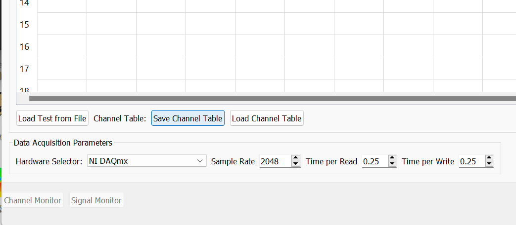
Figure E2.7:Saving out an empty channel table to fill out for the test.
In a real test, we would apply instrumentation to the test article and then record that information in the channel table. In this case, the degrees of freedom names are already stored in the SDynPy System object, we only need to tell Rattlesnake which degrees of freedom to use for excitations and responses. Recall in our code, we specified our responses as nodes 2, 13, 19, and 24 in the Y- direction. We will fill our our channel table with those nodes and directions. We will also put the excitation signal (i.e. force) at node 2, which mirrors what was done in Section 1.2. Note that Rattlesnake will interrogate the SDynPy System object to handle the bookkeeping to determine which System degree of freedom is equivalent to each channel in the Rattlesnake test. Rattlesnake will handle polarity changes is for example, Y- direction is specified in the test whereas Y+ direction was specified in the System object.
We can look back at Chapter 10 to see what needs to be set up in the channel table for a test using a SDynPy System object. We will fill in the Node Number and Node Direction with the node numbers and directions. We will put Virtual in the Physical Device column to specify that a given channel is active. We will put Input in the Feedback Device column. The Type must also be specified, as it will determine the derivative applied to an acquired response channel. We will put the word Acceleration in that column for the response channels. We will put Force in that channel for the excitation signal.
Other columns of the channel table may be filled out to provide additional documentation, but they are not required. For example, we could put units on our data to tell users of the dataset that the data will be in SI units, or we could put comments to describe various aspects of the test. The channel table is shown in Figure E2.8.

Figure E2.8:Channel Table used in the SDynPy Modal Test.
Note that there is no voltage signal in the channel table because the SDynPy system has no knowledge of a shaker model to use in an integration. However, Rattlesnake still needs to know which signals are responses and which signals are inputs, so we must specify those signals in the Feedback Device column of the channel table. It may sound strange to think of “feedback” in terms of a synthetic test, as we are not teeing any signal back to a separate channel on the data acquisition. However, one can think of this as a kind of “virtual” feedback: the signal being applied to the structure as an input when integrating equations of motions is also “fed back” to the user as a response that is measured as an output of the integration.
With the channel table set up, we can now start Rattlesnake and load the channel table. We will again select the Modal Testing environment, click the Load Channel Table button and load our file. Note that we must switch the Hardware Selector from NI DAQmx to SDynPy System Integration... as shown in Figure E2.9.
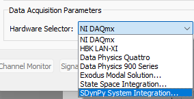
Figure E2.9:Selecting SDynPy System Integration... as the hardware device used in the test.
When this option is selected, a file dialog will appear, and the user must select the file in which the System object was saved. In this case, it is sdynpy_system.npz. An extra parameter Integration Oversample will also appear, which specifies the Sample Rate used by the time integration compared to the sample rate of the test. We will again set the Sample Rate to 5120 Hz, and we will leave the default Integration Oversample factor at 10, which will mean that the time integration will take place at 51200 time steps per second, but the result will be downsampled back to 5120 Hz to provide commonality with other hardware devices. Figure E2.10 shows these settings in the Rattlesnake GUI.
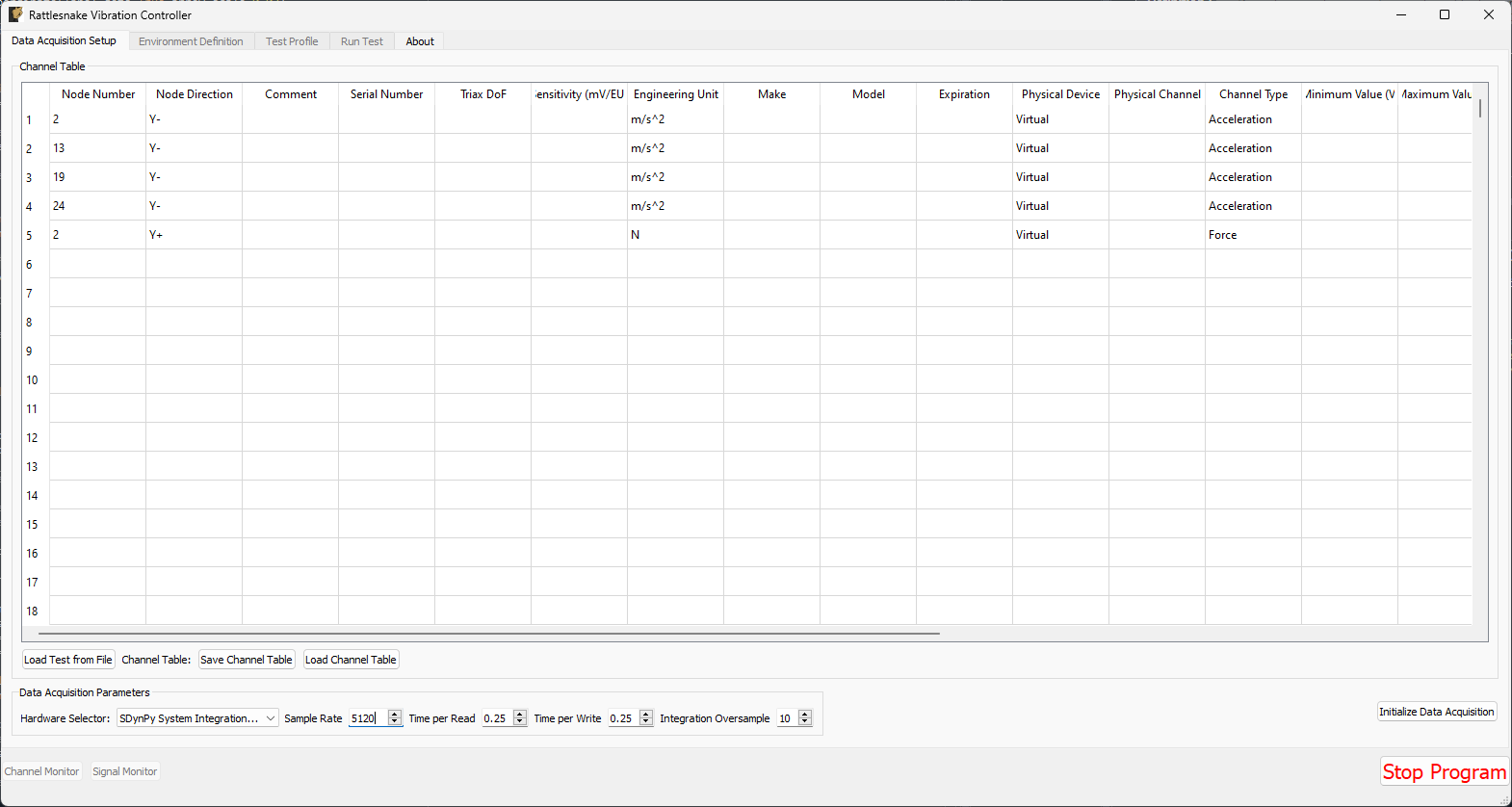
Figure E2.10:Data Acquisition Settings used to perform the Synthetic SDynPy Modal Test.
At this point, we can click the Initialize Data Acquisition button shown in Figure E2.11 to proceed to the next stage of the test.
Figure E2.11:Click the Initialize Data Acquisition button to proceed.
2.2.2Environment Definition for Pseudorandom Excitation
Now we set up the Modal Testing environment parameters. Because we only have one shaker, we can use the Pseudorandom excitation, so we will plan for that.
We will leave the Samples per Frame at its default value. We will change the Number of Averages to 10. We will leave Triggering Type set to Free Run, but we will add a delay of 5 in the Wait for Steady State box, to allow the system to come to steady state, as assumed by the Pseudorandom excitation.
In the Channel Selections box, we select the Force channel as the reference.
In the Signal Generator portion of the window, we select the Pseudorandom tab to set up a Pseudorandom signal. We can truncate the Frequency Range from 10 -- 2000 to remove the large rigid body motion that can occur at low frequency, as well as the portion of the excitation that is in the anti-aliasing filters of the system (note that there are no anti-aliasing filters in the synthetic integration, but it is good practice for when moving to real data acquisition systems). We will set the RMS value to 0.1 V. Note, however, that this will actually be the force level in Newtons due to how the synthetic test is set up.
With these parameters set, we can click the Initialize Environments button to proceed. Figure E2.12 shows these settings in the Rattlesnake GUI.
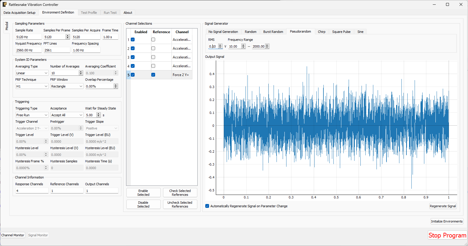
Figure E2.12:Parameters set for the Pseudorandom shaker excitation.
2.2.3Test Profile
We will leave the Test Profile tab empty. Simply click the Initialize Profile button to proceed on this tab.
2.2.4Run Test
We will save the standard modal data file from this test, so we won’t worry about setting up streaming.
To enable the Modal Environment, first click the Arm Data Acquisition button. At this point, the modal environment buttons will become enabled, as shown in Figure E2.13
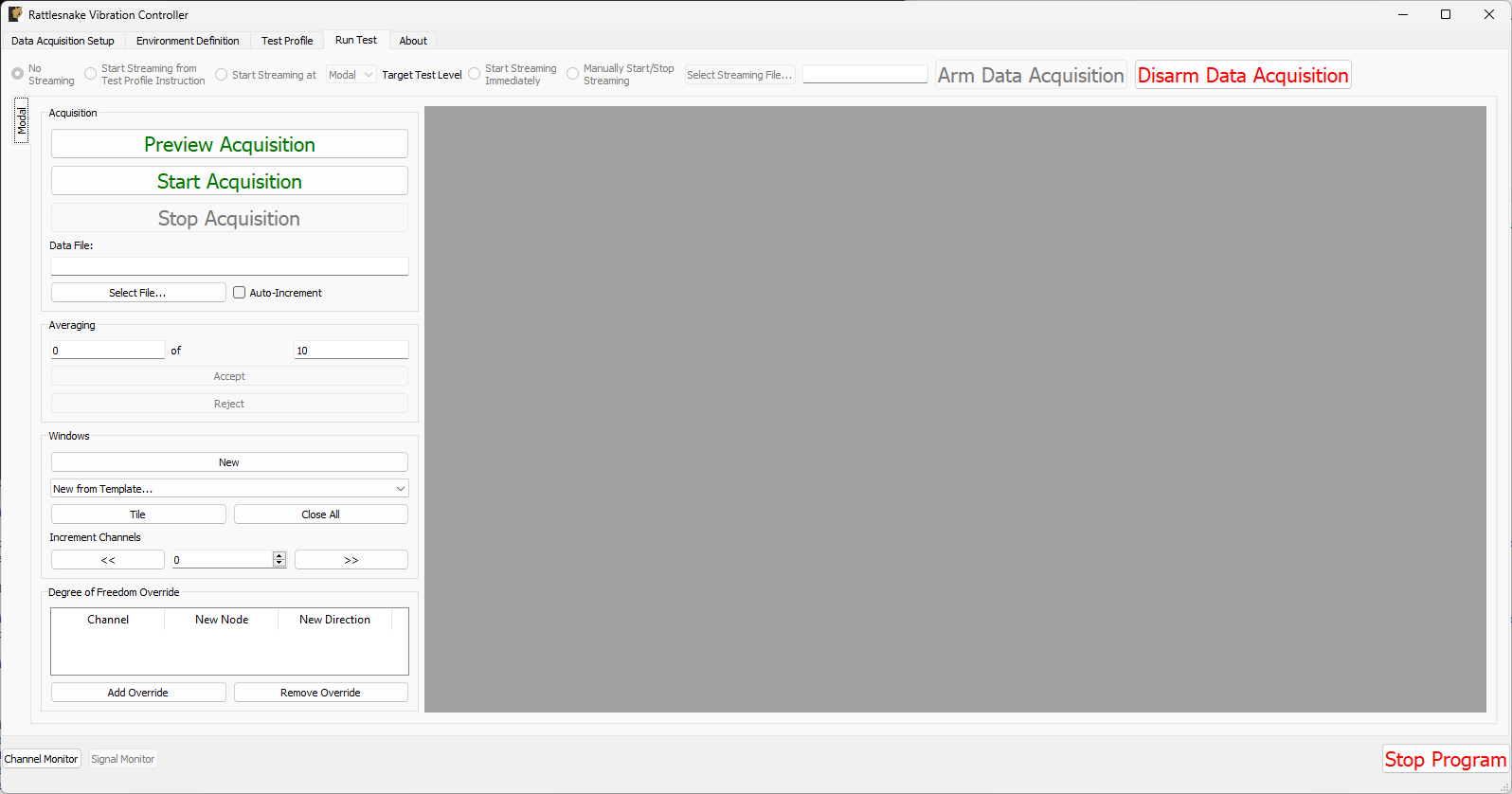
Figure E2.13:Run Test tab with data acquisition armed
Next we can set up data display windows. We will use the New from Template... dropdown menu to create Drive Point (Imaginary), Drive Point Coherence, and Reference Autospectrum channels. We will also manually create 5 windows by clicking the New button, and set them to visualize the time histories for each channel; these will help us determine if we need to change the trigger settings, frame length, or add a window. Clicking the Tile button will expand the windows to fill up the available space. Figure E2.14 shows the result of these operations.
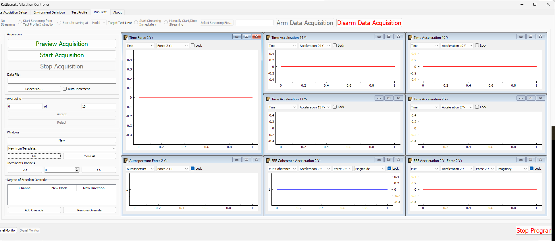
Figure E2.14:Run Test tab with modal windows created.
We can then Preview Acquisition to see how the test parameters look. Data will take a few seconds to appear after the shaker starts due to the Wait for Steady State parameter that was set. Ideally if the pseudorandom excitation has reached steady state, we should see no appreciable difference between the time response of measurement frames, as the exact same signal is being applied and exact same responses are being measured. This is shown in Figure E2.15. Note that due to there being no excitation signal past 2000 Hz and below 10 Hz, the FRF values may be quite large in those frequency ranges, because the computation is essentially dividing by zero at those frequency lines. You may need to adjust the limits of the Y-axis appropriately to visualize the data from 10--2000 Hz.
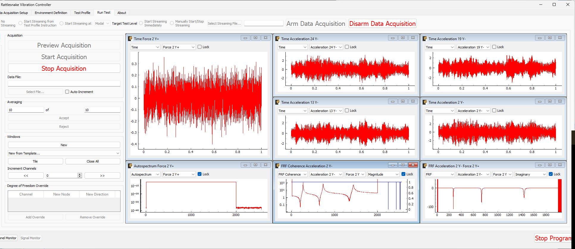
Figure E2.15:Previewing the data acquisition with the pseudorandom excitation.
If we are happy with the preview, we can move to Start Acquisition. We must first define a file to save the data, which we will call beam_shaker_pseudorandom.nc4. This is shown in Figure E2.16. The measurement and shakers should stop automatically when the requested number of averages have been acquired.
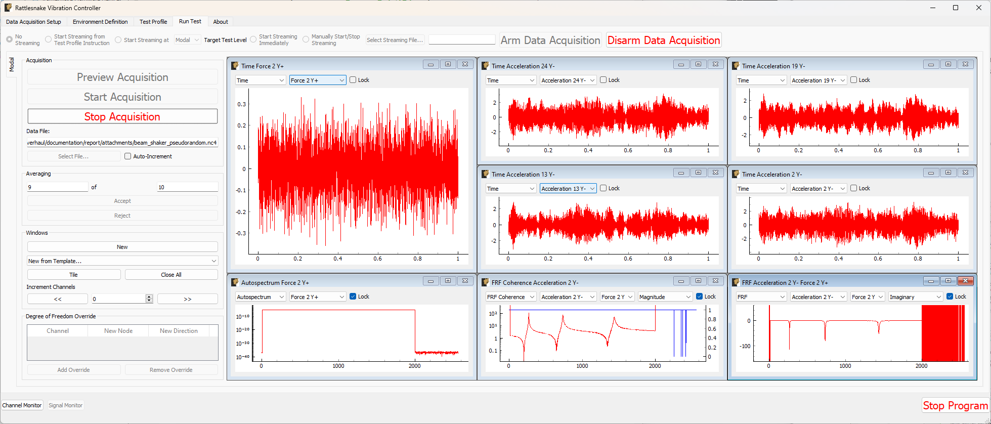
Figure E2.16:Acquiring the pseudorandom modal data.
2.2.5Other Shaker Excitation Types
We will return to the Environment Definition tab and set up a Burst Random test. We don’t know exactly how long the structure will take to ring down, so we will set the Samples Per Frame value to 15360 to achieve a 3 second frame. We will set the Number of Averages to 30. We will set the Triggering Type to First Frame, remove the Wait for Steady State value, and set the Trigger Channel to the force channel with a Pretrigger of 1%. We will set the Trigger Level to 0.1%, the Hysteresis Level to half that value, and the Hysteresis Frame % to 25%. Note that because there is no “sensitivity” value that translates voltage to engineering unit in the synthetic case, the two values are treated equally.
In the Signal Generator section, we will select a Burst Random signal and set the On Percentage to 33% to provide a 1 second burst and 2 second ring down. We will keep the other parameters the same as our previous Pseudorandom test.
Figure E2.17 shows the parameters in the Rattlesnake GUI. Click the Initialize Environments button to proceed, and return to the Run Test tab.
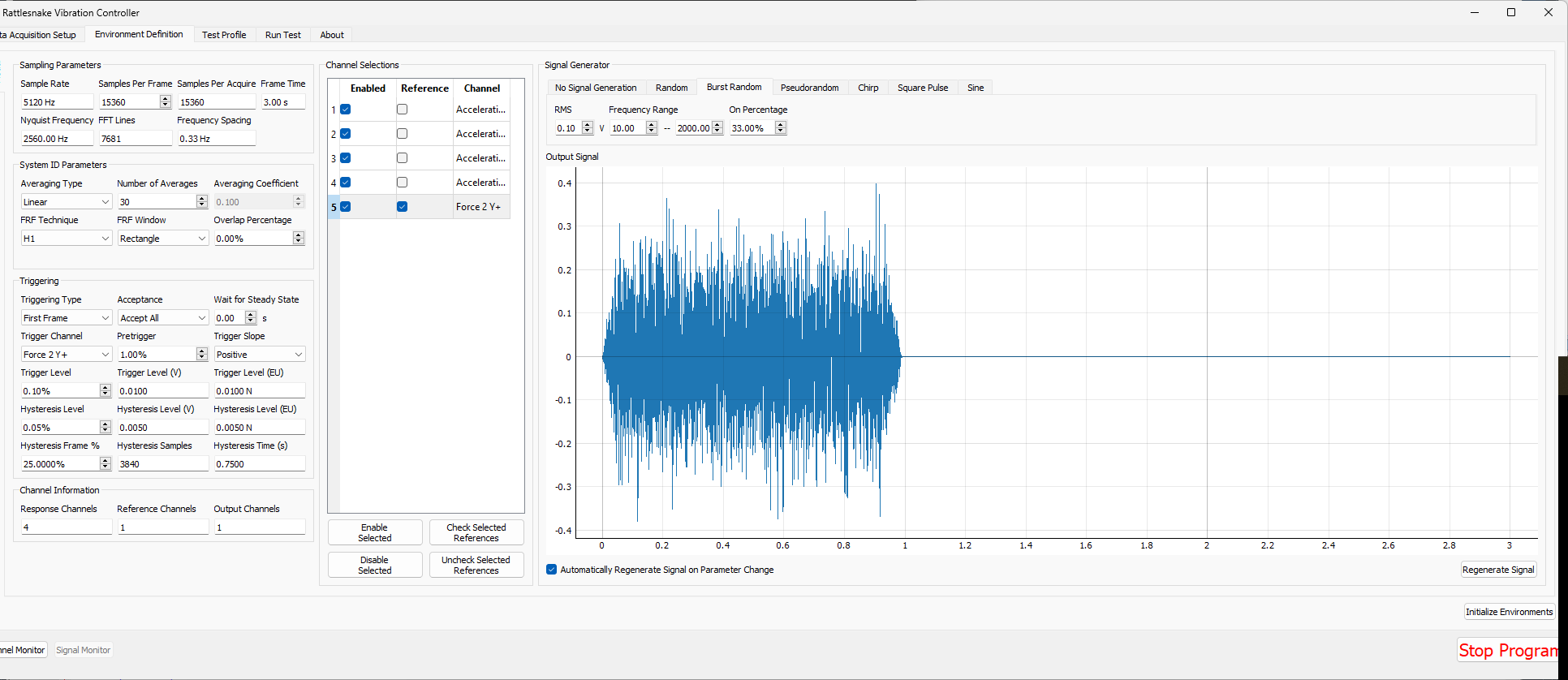
Figure E2.17:Test parameters for the Burst Random excitation
We can preview the signal by clicking the Preview Acquisition button to ensure that the triggering has been set up correctly and the signals ring down appropriately. Figure E2.18 shows the previewed data.
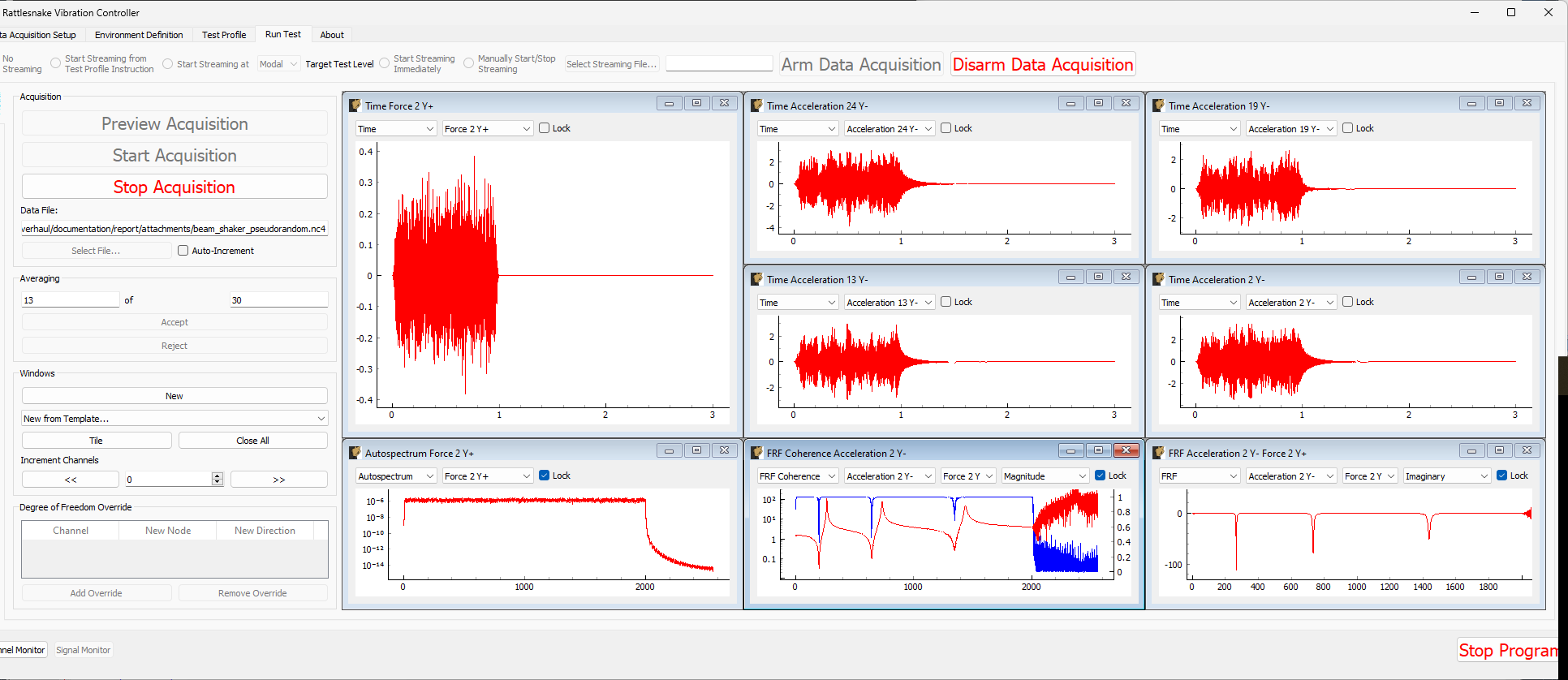
Figure E2.18:Previewing the measurement with the initial parameter set.
Looking at the preview data, the damping is such that the that the structure stops ringing by approximately 1/2 second after the burst finishes. Let’s therefore Stop Acquisition, Disarm Data Acquisition, and return to the Environment Definition tab. We will update the Samples Per Frame value to 5120 to achieve a 1 second measurement frame. We will also change the burst On Percentage to 50%.
Figure E2.19 shows the updated parameters in the Rattlesnake GUI. Click the Initialize Environments button to confirm these settings, and return to the Run Test tab.
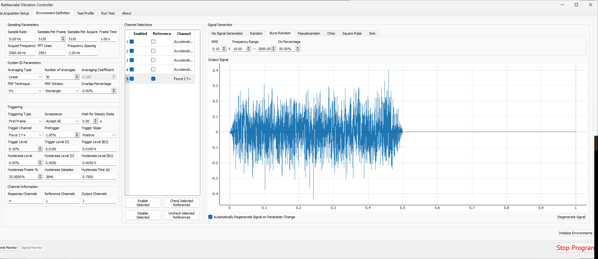
Figure E2.19:Updated burst random parameters after previewing the initial guess at the parameters.
We can then preview this new configuration by Arm Data Acquisition and Start Preview. The results are shown in Figure E2.20. This configuration looks good and runs 3x faster, so we will keep it.
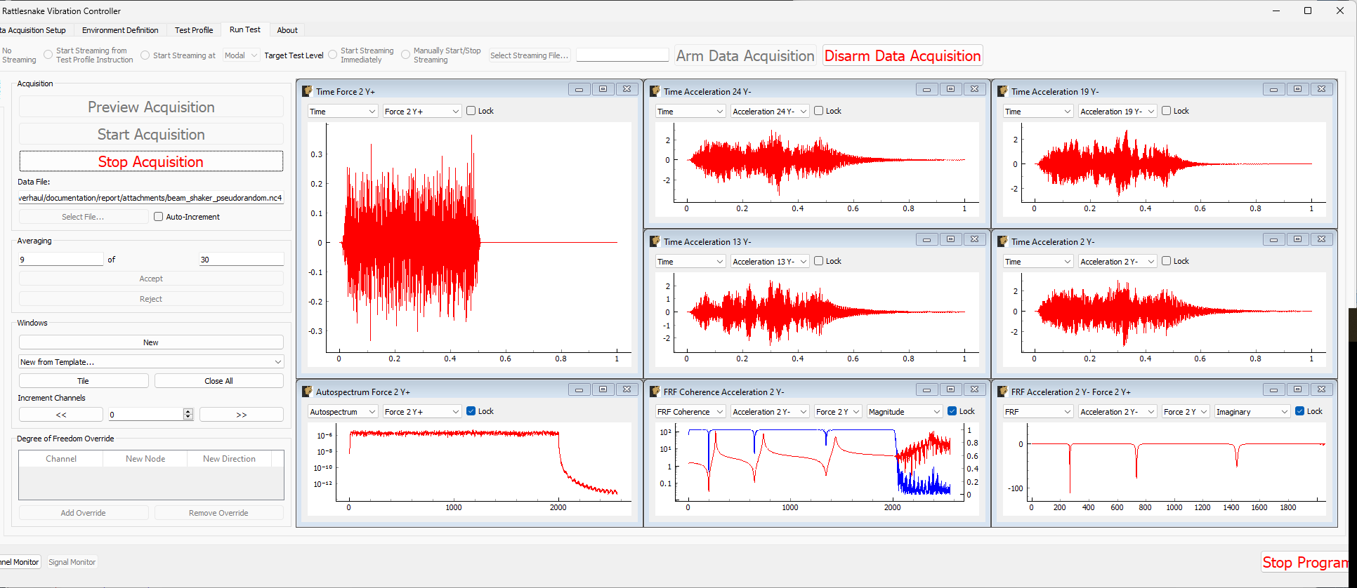
Figure E2.20:Previewing the measurement with the updated parameter set.
Press the Stop Acquisition button to stop the preview, set a file to store the results to (beam_shaker_burst.nc4) and Start Acquisition. The acquisition should stop automatically when 30 averages are obtained. Figure E2.21 shows the measurement midway through acquisition.
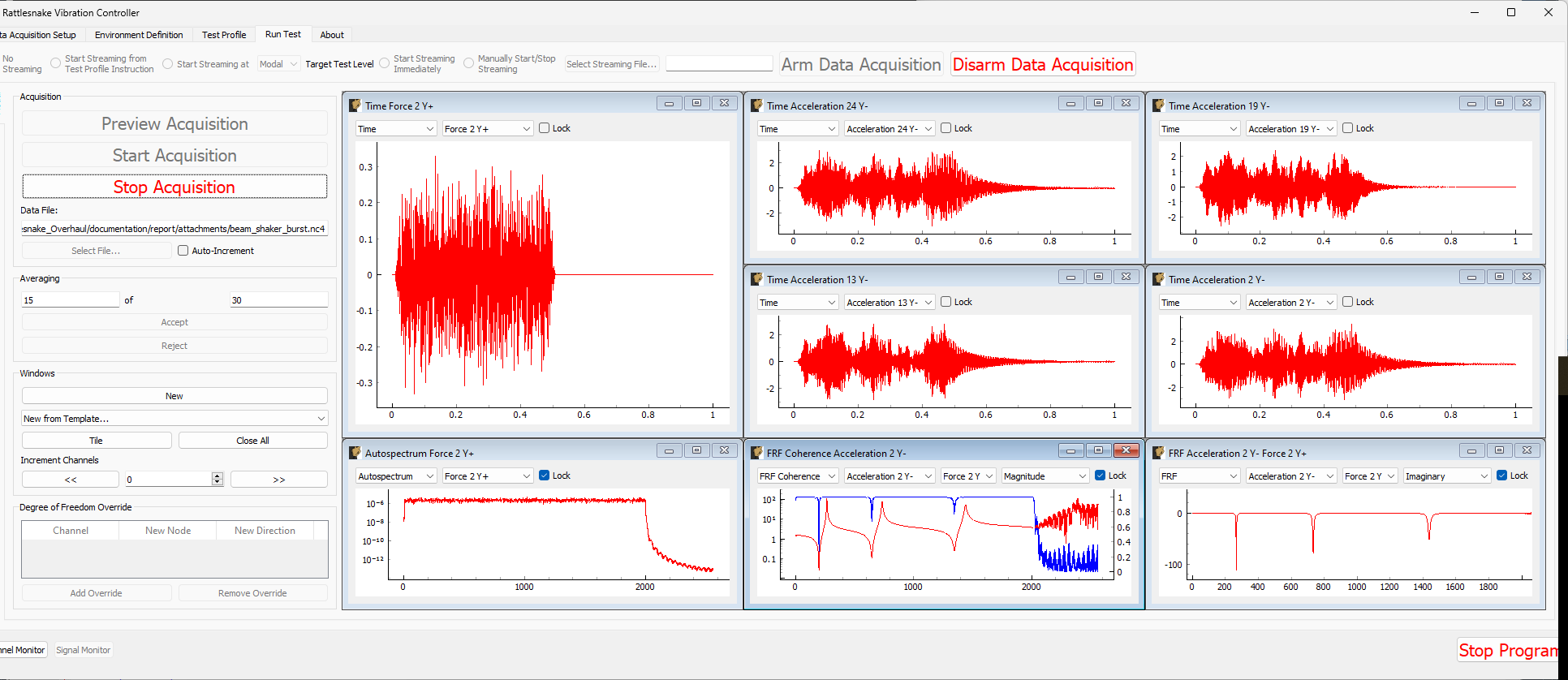
Figure E2.21:Acquiring the burst random data
2.2.6Analyzing Modal Data
To analyze these data, we will again use SDynPy[1], which is an open-source Python-based structural dynamics toolset. We will focus on the Burst Random test data, but analyzing the Pseudorandom data should be very similar. A Python script containing the commands is attached to this document as a .txt file[2], which can be transformed to a Python file by renaming the .txt to .py.
SDynPy is well-integrated with Rattlesnake, making it trivial to load in data from a Rattlesnake test. For example, reading in a modal dataset with SDynPy looks like:
# Import SDynPy and Numpy
import sdynpy as sdpy
import numpy as np

# Read a rattlesnake file using `read_modal_data`
time_data, frfs, coherence, channel_table = sdpy.rattlesnake.read_modal_data(
    'beam_hammer_impact_0000.nc4')
We can plot the data easily using SDynPy’s plotting functionality:
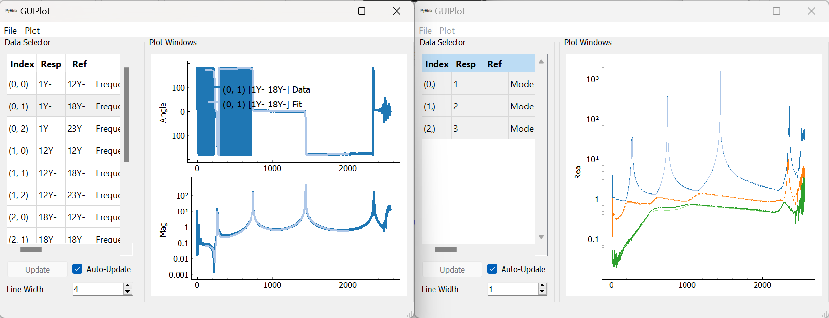
frfs.plot(one_axis=False,subplots_kwargs={'layout':'constrained'})The results of this command are shown in Figure E2.22.
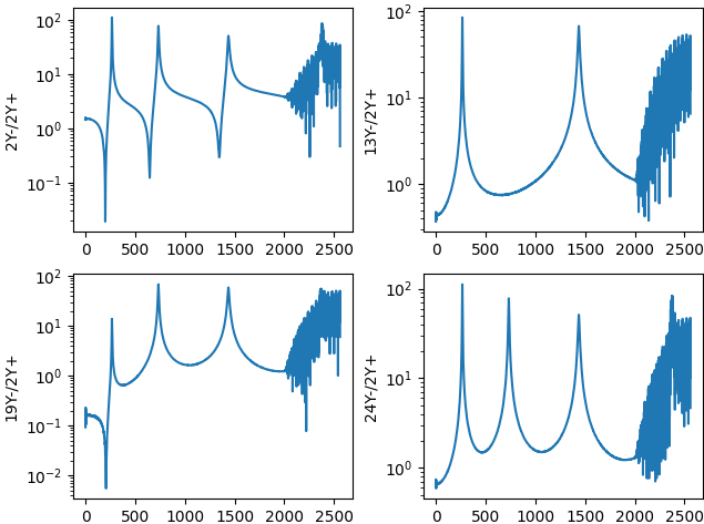
Figure E2.22:Frequency response functions plotted in SDynPy from the modal impact test.
Ideally we would like to plot mode shapes of this test, so as a first step towards that goal we will construct a test geometry. This contains nodes, coordinate systems, and optionally tracelines or elements. We can construct nodes with the ID numbers given in the test and coordinates specified by each node’s position along the beam. Here we construct and print a node_array in SDynPy
nodes = sdpy.node_array(id = [2,13,19,24],
                        coordinate = [[1,0,0],
                                      [12,0,0],
                                      [18,0,0],
                                      [23,0,0]])
print(nodes)
which has output
Index,     ID,        X,        Y,        Z, DefCS, DisCS
 (0,),      2,    1.000,    0.000,    0.000,     1,     1
 (1,),     13,   12.000,    0.000,    0.000,     1,     1
 (2,),     19,   18.000,    0.000,    0.000,     1,     1
 (3,),     24,   23.000,    0.000,    0.000,     1,     1
We will do similarly with a global coordinate system
css = sdpy.coordinate_system_array(id=1,name='global')
print(css)
which has output
Index,     ID,                 Name, Color,       Type
   (),      1,               global,     1,  Cartesian
We can then construct a Geometry object. We will then add a traceline to connect the nodes together. We will then plot the geometry.
geometry = sdpy.Geometry(nodes,css)
geometry.add_traceline([2,13,19,24])
geometry.plot()
The plotted geometry is shown in Figure E2.23.
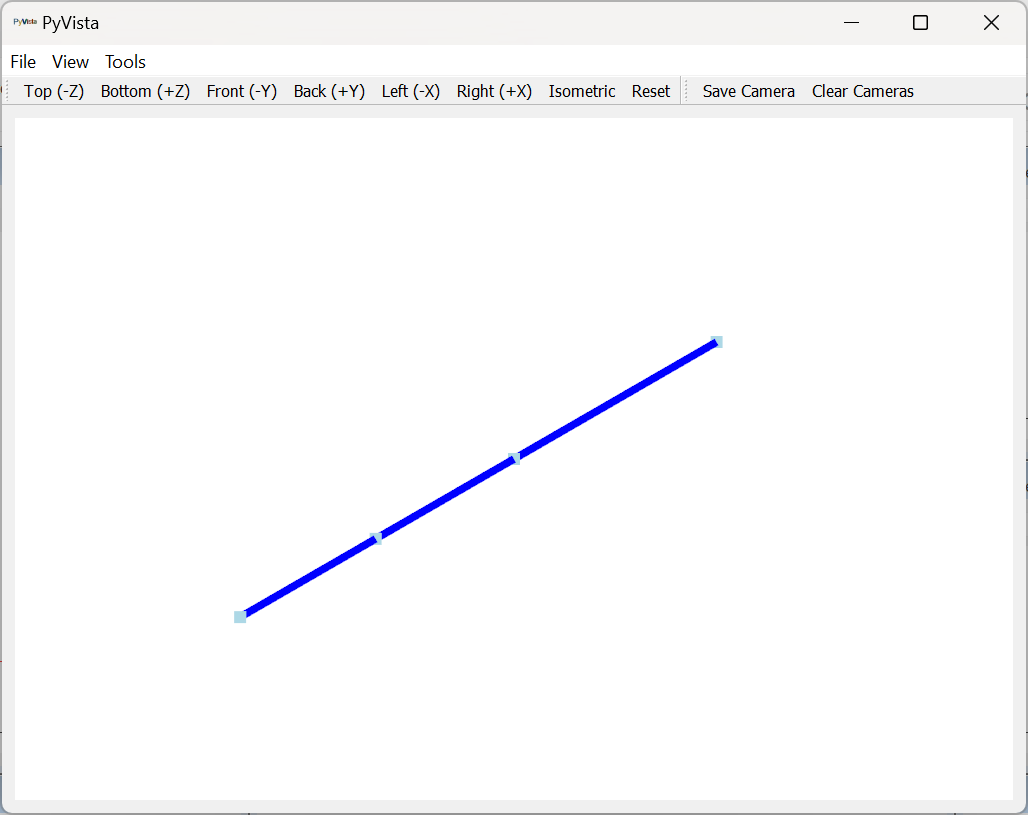
Figure E2.23:Geometry used to plot mode shapes in the modal test.
Note that an alternative way to construct the geometry would have been to use the geometry output directly from the sdynpy.System.beam function, and remove any nodes that were not defined in the test.
Now that we have a geometry, we can fit modes and plot mode shapes. We will only fit up to approximately 2000 Hz, which was the maximum frequency of the excitation. We will use the PolyPy_GUI in SDynPy to do the mode fits. We can add our geometry directly to the fitter by assigning to the geometry attribute.
ppgui = sdpy.PolyPy_GUI(frfs)
ppgui.geometry = geometry
We can select frequency ranges and polynomial orders to solve for, then click Compute Stabilization to proceed, as shown in Figure E2.24.
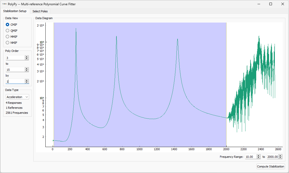
Figure E2.24:Setting up frequency ranges and polynomial orders in PolyPy.
We can then select stable poles from the diagram and plot resynthesized FRFs or mode indicator functions, shown in Figure E2.25.
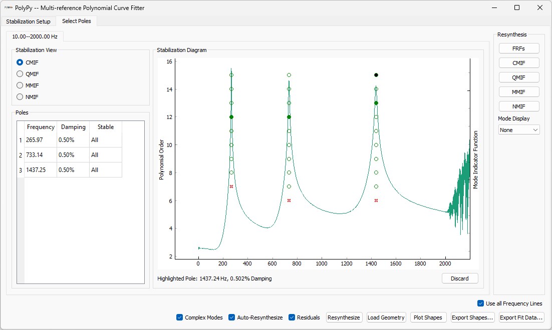
(a)Selecting stable poles
(b)Visualizing resynthesized FRFs
Figure E2.25:Selecting stable poles and visualizing resynthesized FRFs.
We can then plot mode shapes from the test. Note that with only four sensors, our mode shapes will not be very highly resolved; however, they clearly correspond to the first three bending modes of the beam. The first mode shape is shown in Figure E2.26.
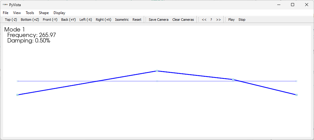
Figure E2.26:First mode shape fit to the modal data from the impact test.
2.3Running a Synthetic Vibration Test with Rattlesnake
Now we will demonstrate how we can simulate a controlled vibration test with Rattlesnake. We will demonstrate both Random and Transient vibration control in this section.
2.3.1Setting up the Channel Table
We will now set up our vibration test. We add a second shaker to the other end of the beam using a second drive at node 24, in addition to the drive at node 2 used in the modal test. We will now have two force channels applied to the structure. Note that the control channels in the test must be in the same order as the channels in the specification that we constructed in Section 2.1.4.
Our channel table now looks like Figure E2.27.

Figure E2.27:Channel table for the random vibration test setup
2.3.2Setting up the Random Vibration Test
Now that the specification and channel table are set up, we will set up our random vibration test. We will open Rattlesnake and select the MIMO Random Vibration environment as shown in Figure E2.28.
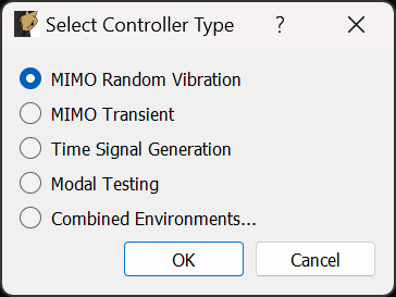
Figure E2.28:Selecting the MIMO Random Vibration environment
On the Data Acquisition Setup tab, we will Load Channel Table to import our Excel channel spreadsheet. We will set the Hardware Selector to SDynPy System Integration... and select our system file sdynpy_system.npz, as well as set the sample Sample Rate to 5120. The other parameters can be left at their default values. Figure E2.29 shows these parameters.
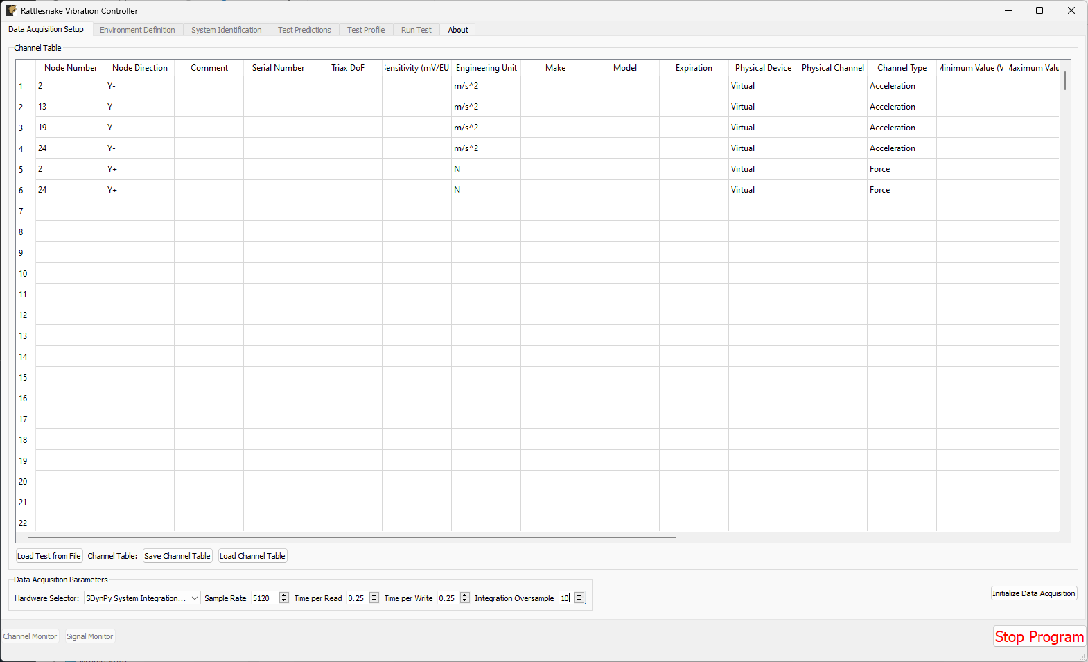
Figure E2.29:Data acquisition setup for the vibration tests.
Click the Initialize Data Acquisition button to proceed.
On the Environment Definition tab, we will keep the Samples Per Frame set to 5120, which is consistent with the parameters used to construct the specification. In the Control Python Script section, we will click Load to select a control law. We will use the control_laws.py file, which is located in the control_laws folder of the main Rattlesnake directory. In the Control Python Function drop-down, we will select pseudoinverse_control.
In the Control Channels section, we will select all four acceleration channels, which we will use to control to the environment.
Finally we will click the Load Spec button and navigate to our random specification file random_specification.npz from SDynPy. The specification should then appear in the plots.
With these parameters selected, we can click the Initialize Environments button to proceed. Figure E2.30 shows the parameters in the Rattlesnake GUI.
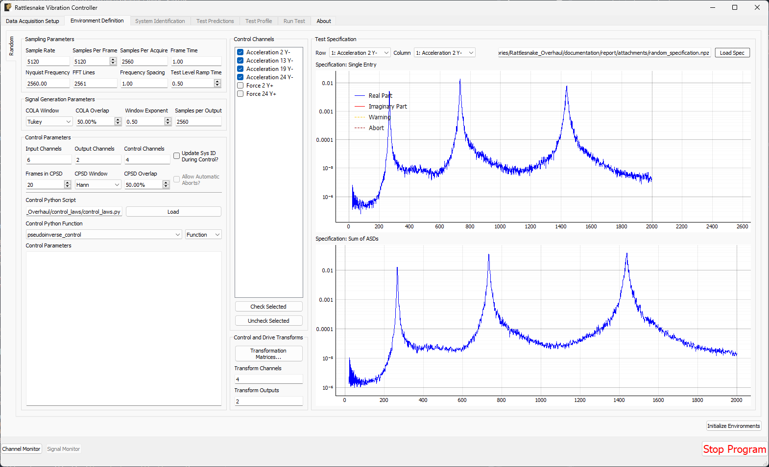
Figure E2.30:Random vibration parameters specified in the Rattlesnake GUI.
At this point, we must run the System Identification phase of the controller. We will set the Level to 0.1 V RMS, then click Start to start the system identification. A noise floor check will first be run (noise will be zero for a synthetic test), then the system identification follows. Rattlesnake will determine the transfer functions between the two shaker drive forces and the four accelerometer channels. When the specified number of averages have been obtained, the System Identification will stop automatically. Figure E2.31 shows the system identification phase of the controller.
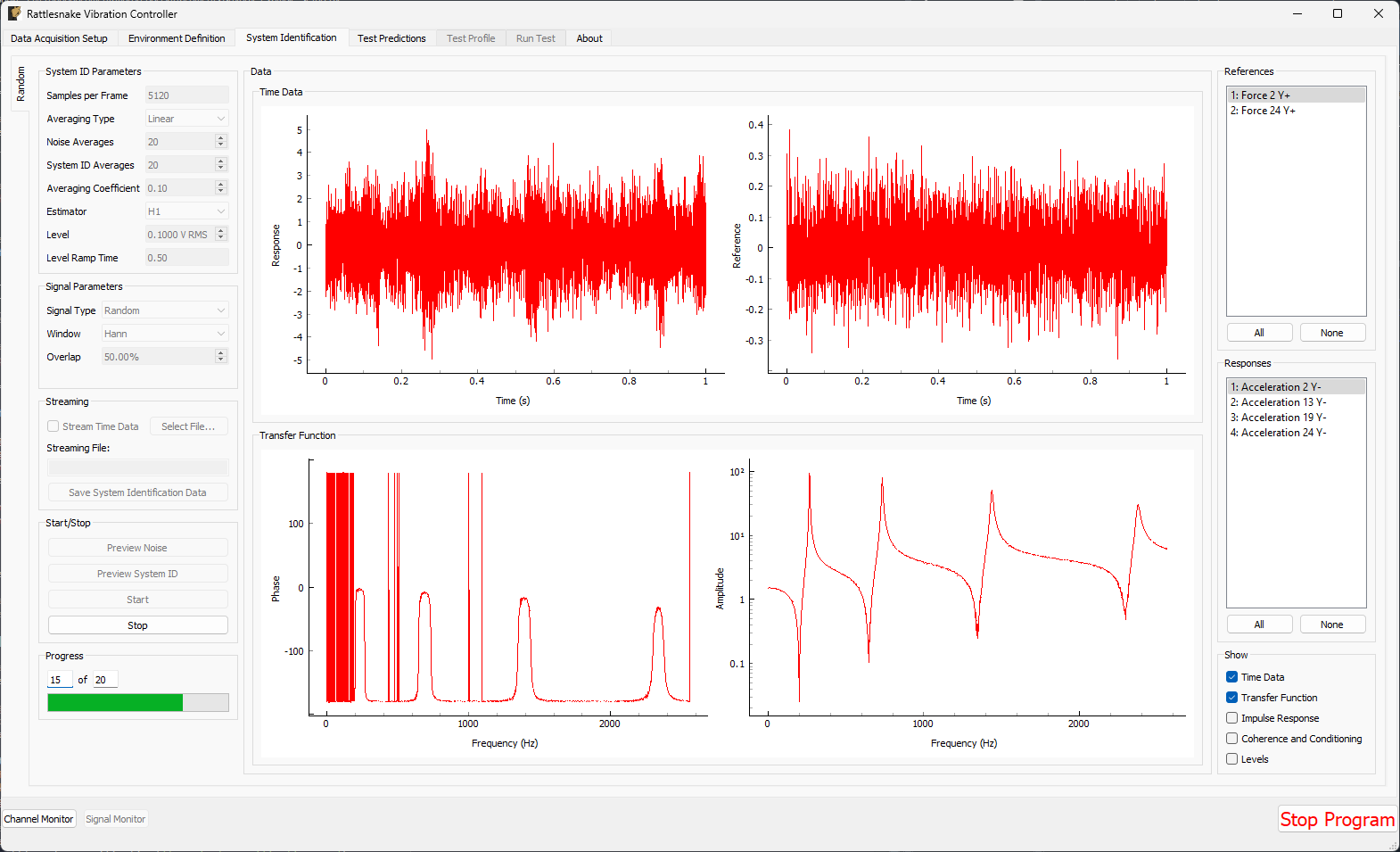
Figure E2.31:System identification for the Random Vibration environment.
On the Test Prediction tab, Rattlesnake will make predictions of the voltage that it will need to output to achieve the control specified, as well as the responses predicted to be obtained. Here it is important to note that the output signals are not too large for the shakers, though with synthetic data, there is no real risk of damaging anything if they are too large. Figure E2.32 shows the predictions for this test.
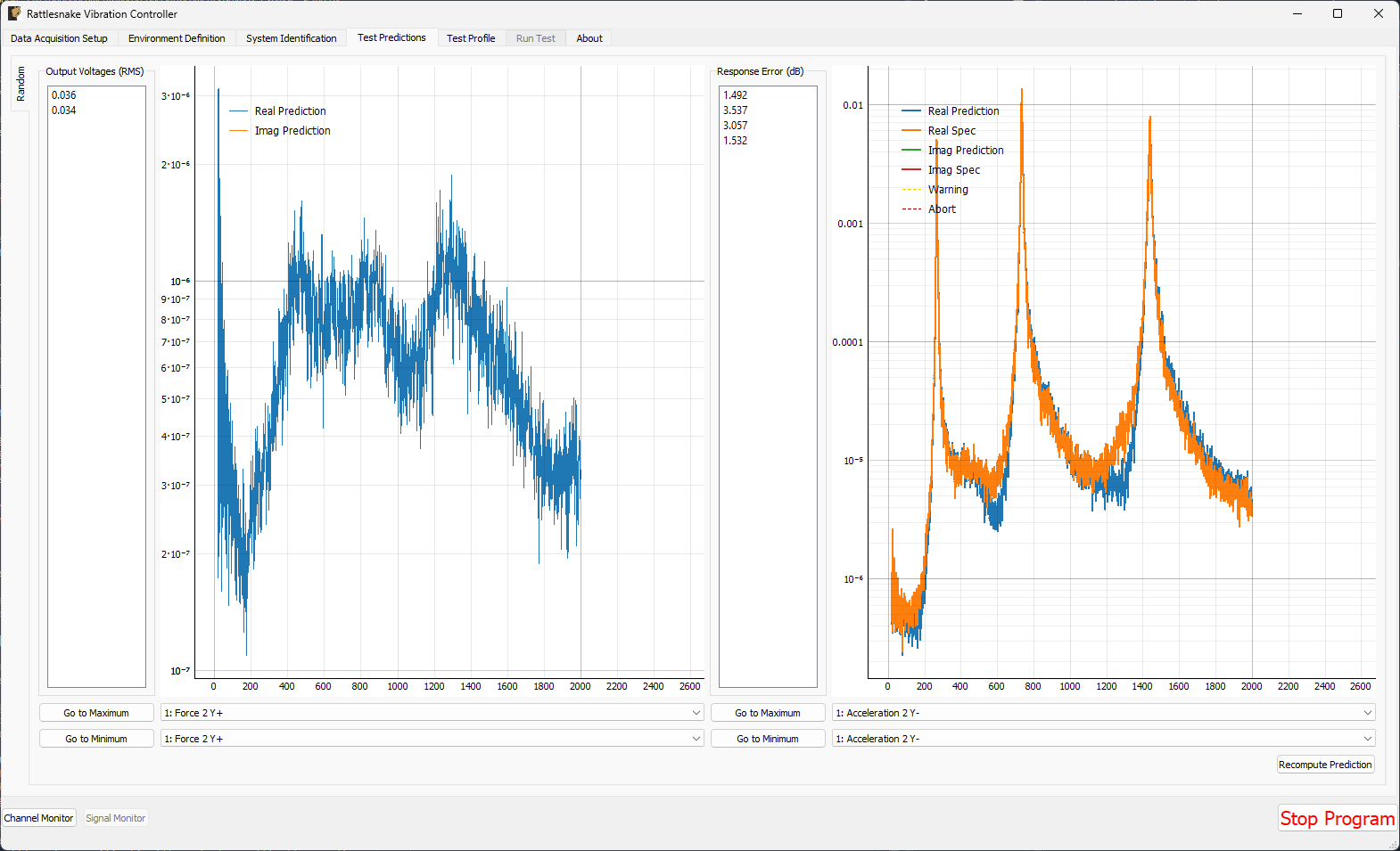
Figure E2.32:Test predictions for the random vibration environment
If the predictions look good, we can proceed to the Test Profile tab, which we will again leave blank and click the Initialize Test Profile button to proceed to the Run Test tab.
2.3.3Running a Random Vibration Test
On the Run Test tab, we see a different interface than the one we saw for the modal test. We can click the Arm Data Acquisition button to enable the Random environment.
To start, we will set the Current Test Level to -12 dB to ensure when we start the test we don’t break anything (again, a best practice; there is no risk to break anything with a synthetic test). We will then step up slowly to the full 0 dB level test.
We can then click the Start Environment button to start the test.
As the test is running, the main Rattlesnake interface will show the sum of APSDs, which is the trace of the CPSD matrix and can be thought of as an average response of the test (Figure E2.33). To visualize individual channels, windows can be created in the Data Display section of the window (Figure E2.34).
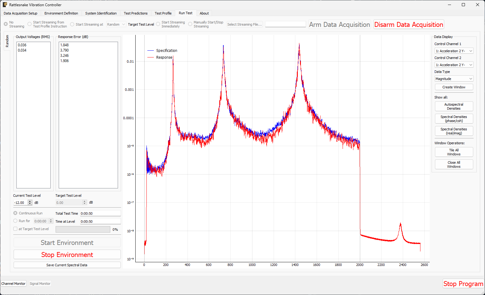
Figure E2.33:Rattlesnake GUI showing the average test response
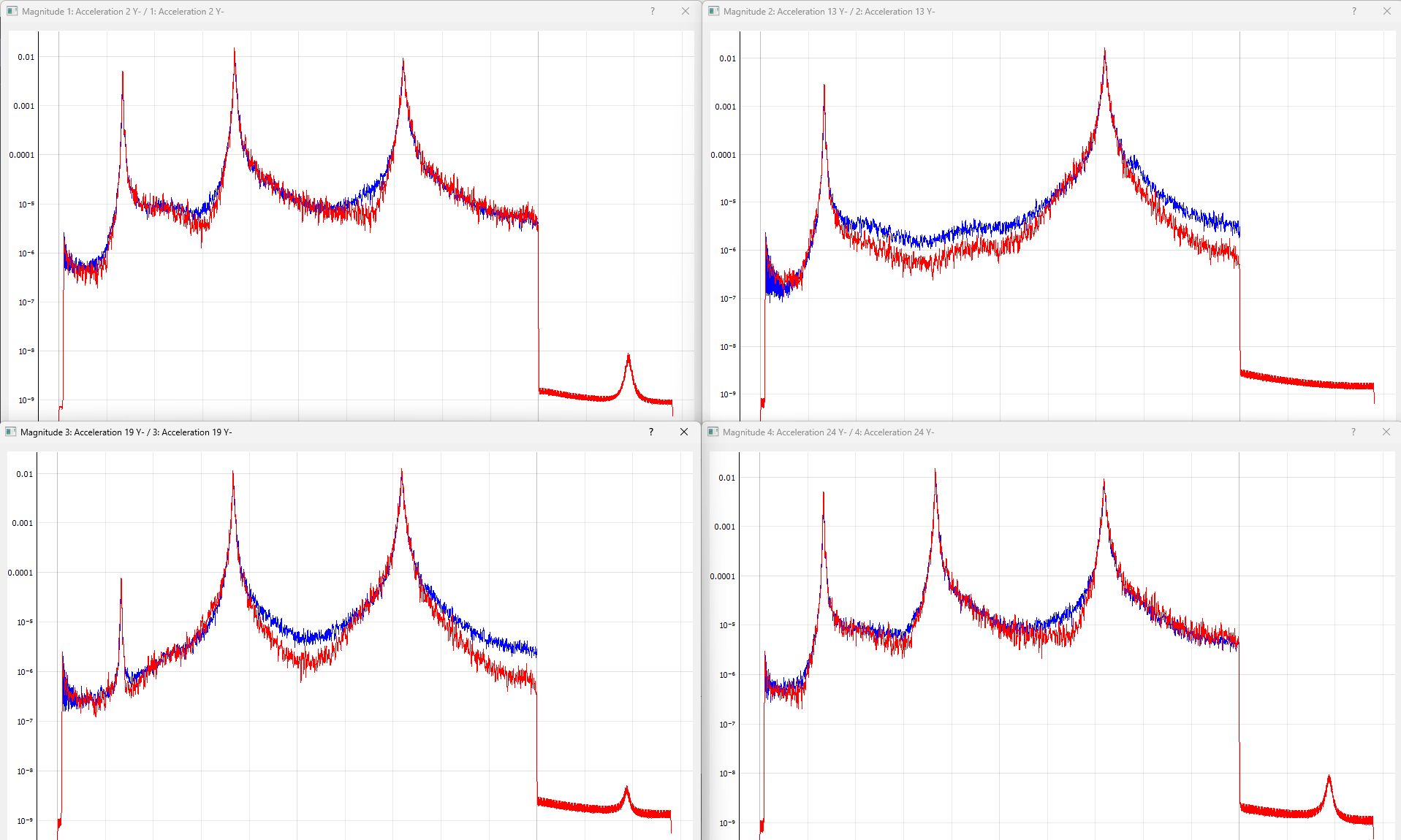
Figure E2.34:Individual channel APSDs showing how well each channel is matching the test level.
If the controller is controlling sufficiently well, we can step up the level to 0 dB for the amount of time specified by the test. Clearly, Rattlesnake has obtained relatively good control for this test.
To save data from the test, we can either stream time data using the same approach used previously, or we can simply use the Save Current Spectral Data to save out the current realizations of the control CPSDs, which we will call random_vibration_spectral_results.nc4. This is the quickest way to do comparisons between the specification and the control achieved. We can load this file with SDynPy and use SDynPy to make comparisons between the test and specification. The results are shown in Figure E2.35.
control, spec, drives = sdpy.rattlesnake.read_random_spectral_data(
    'random_vibration_spectral_results.nc4')
spec = spec.extract_elements_by_abscissa(20,2000)
control = control.extract_elements_by_abscissa(20,2000)
spec.error_summary(figure_kwargs={'figsize':(10,6)},Control=control)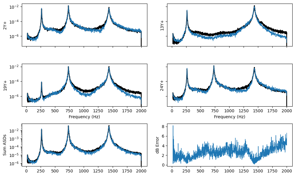
Figure E2.35:Error summary between the test and specification for the random vibration control.
We can then Stop Environment, Disarm Data Acquisition and close the software.
2.3.4Setting up the Transient Vibration Test
The last demonstration will show how we can perform a MIMO Transient environment test. Open Rattlesnake and select the MIMO Transient environment as shown in Figure E2.36.
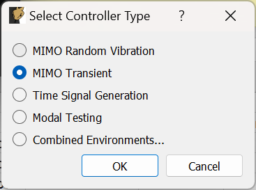
Figure E2.36:Selecting the MIMO Transient environment
We will set the Data Acquisition Setup tab identical to what was used before, as shown in Figure E2.29. Click the Initialize Data Acquisition button to proceed.
On the Environment Definition tab, we will again Load a control law file. This time we will load the transient_control_laws.py file, which contains transient control laws for Rattlesnake. We will select the pseudoinverse_control function.
In the Control Channels section, we will again select all four accelerometer channels as the control channels.
Finally, we will select the Load Signal button to load in our specification file transient_specification.npz. Figure E2.37 shows these parameters set in the Rattlesnake GUI. With these parameters set, we will click the Initialize Environments button to proceed.
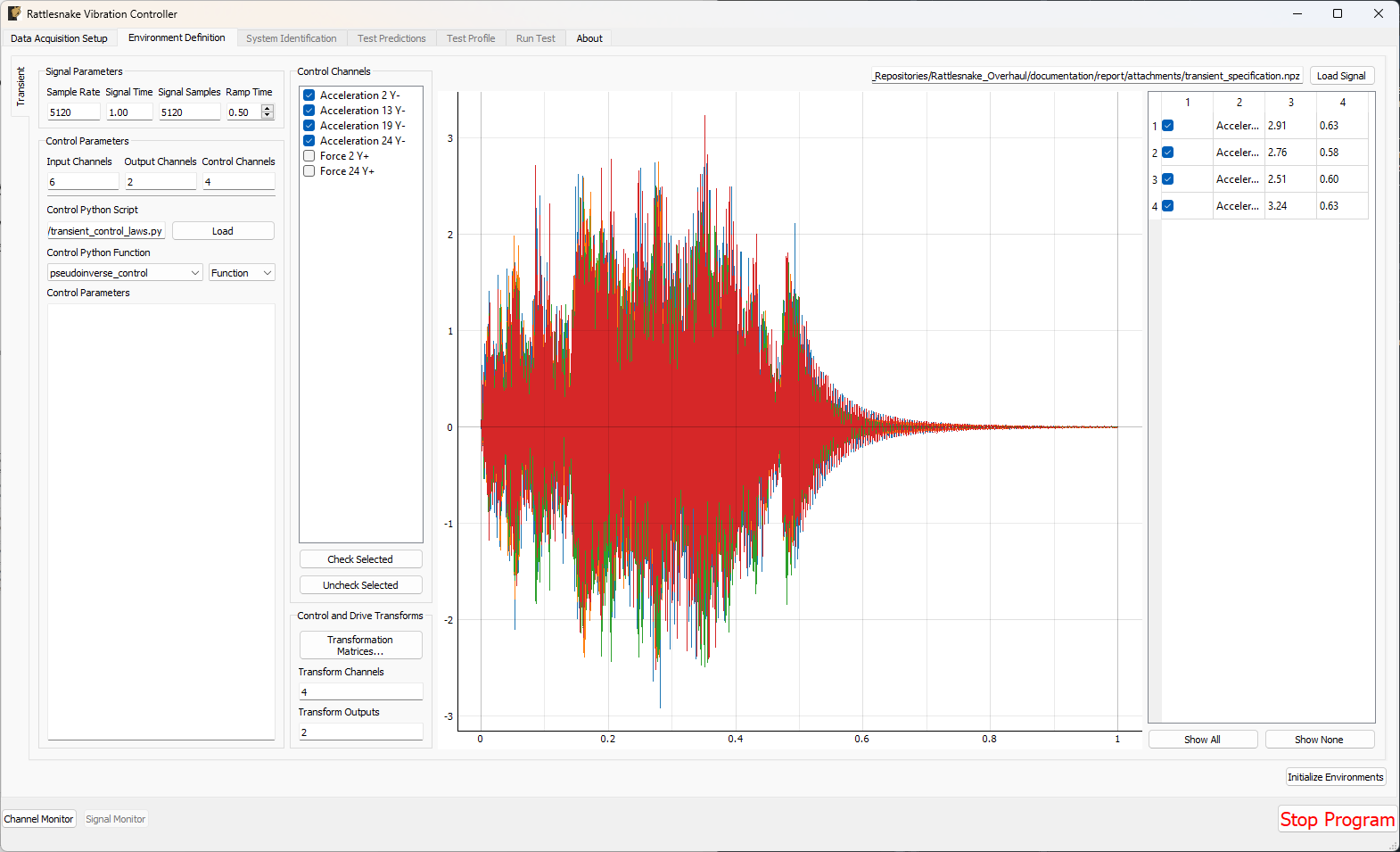
Figure E2.37:Parameters set for the Transient environment in the Rattlesnake GUI.
The Transient environment will also need to perform a System Identification. Again set the Level to 0.1 V RMS and click Start to start the noise floor and system identification. Here it may be useful to look at the Impulse Response, as that is useful to understand how transient control will be performed. This is shown in Figure E2.38.
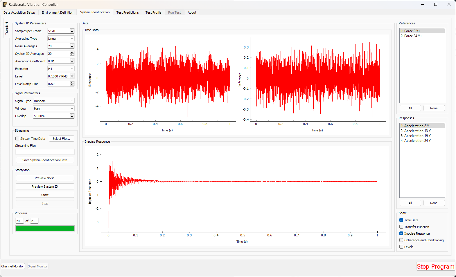
Figure E2.38:System Identification for the Transient environment with Impulse Response function shown.
Once the system identification has been performed, Rattlesnake will again make a prediction as to the results of the test and show it on the Test Predictions tab. It will show the peak signal it aims to output, as well as the response it predicts that it will get compared to the desired response. Figure E2.39 shows these predictions.

Figure E2.39:Test predictions and voltage that will be output for the transient control.
We can then proceed to the Test Profile tab, click the Initialize Profile button, and we are ready to run the test.
2.3.5Running a Transient Test
We can now click the Arm Data Acquisition button to enable the Transient control functionality. We can set the Signal Level to -12 dB to start so we don’t break anything when we run (again, a best practice; there is no risk to break anything with a synthetic test). If it runs successfully, then we can step back up to full level.
Rattlesnake will identify the control signal as it comes through the data acquisition and surround it with a box, as shown in Figure E2.40.
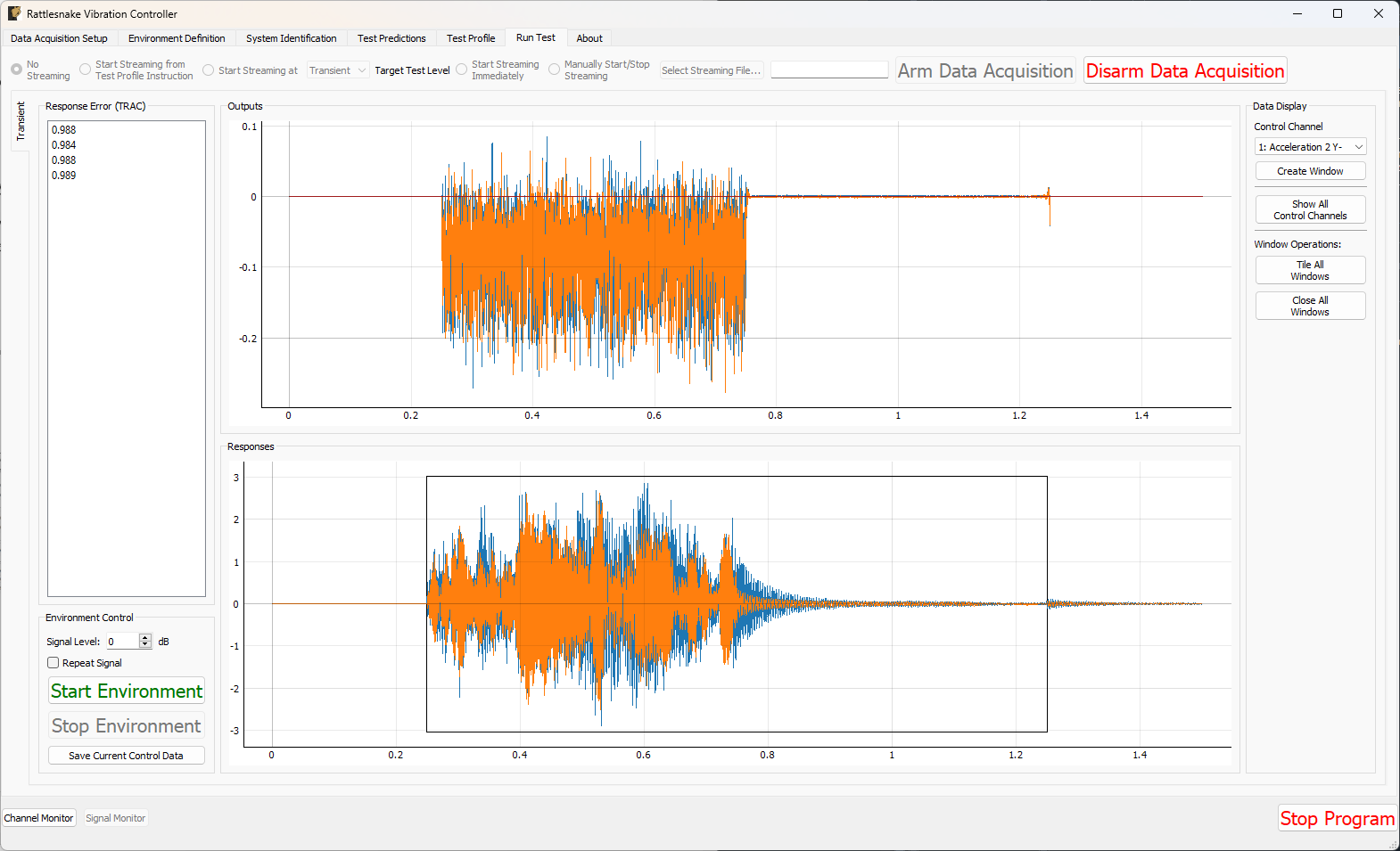
Figure E2.40:Running the transient control with the control signal identified.
To visualize individual channels, new windows can be created in the Data Display portion of the window. The four control channels can be seen in Figure E2.41
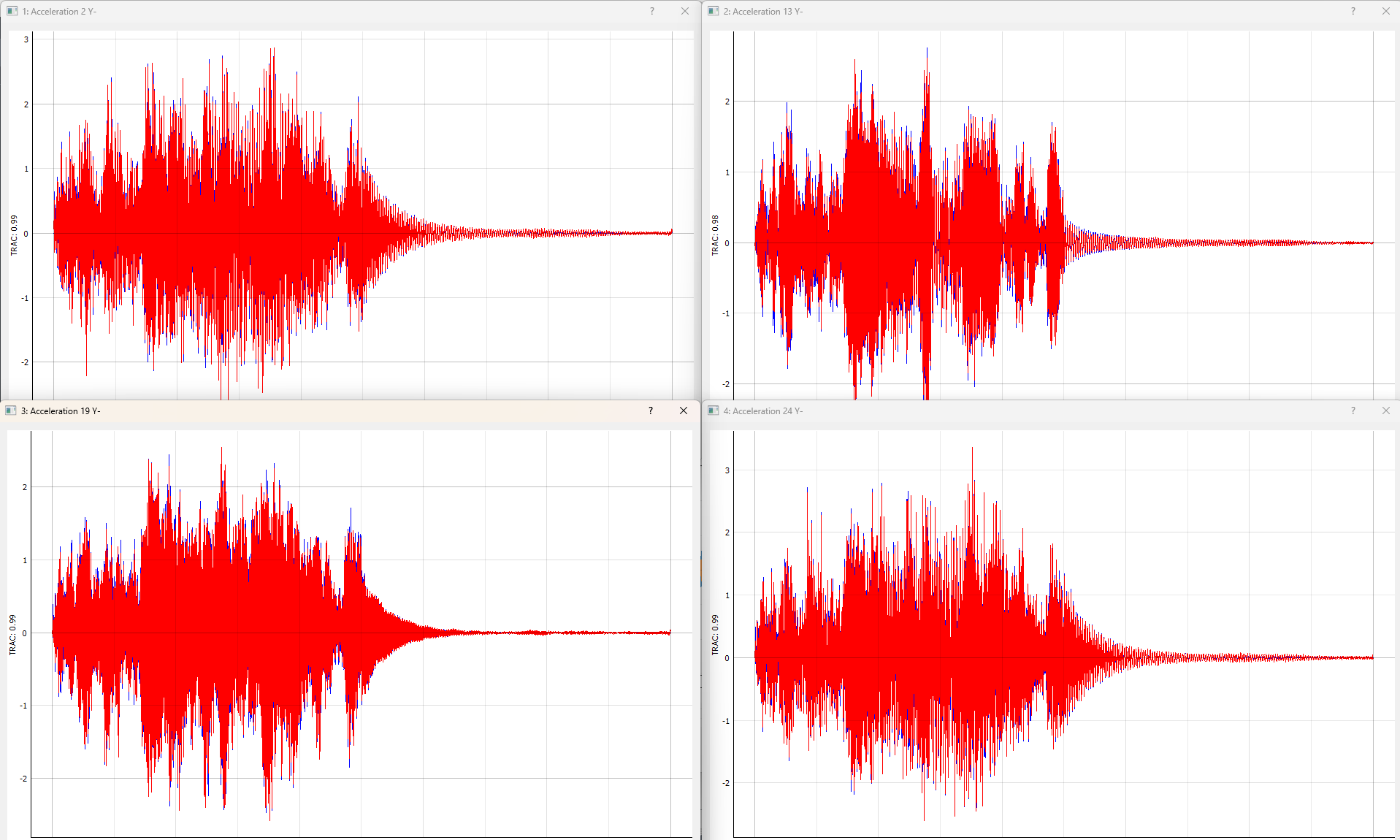
Figure E2.41:Control achieved on each control channel in the Transient vibration test.
To save out data, we can click the Save Current Control Data button. We will save the data to the file transient_vibration_control_results.nc4. This can be loaded into SDynPy to do comparisons to the desired signal. These results are shown in Figure E2.42.
control, specification, drives = sdpy.rattlesnake.read_transient_control_data(
    'transient_vibration_control_results.nc4')

ax = specification.plot(
    one_axis=False, plot_kwargs = {'linewidth':0.5},
    subplots_kwargs = {'figsize':(10,6),'sharex':True,'sharey':True})
for a,c in zip(ax.flatten(),control):
    c.plot(a,plot_kwargs = {'linewidth':0.5})
# Zoom in on a specific portion
a.set_xlim(0.45,0.48)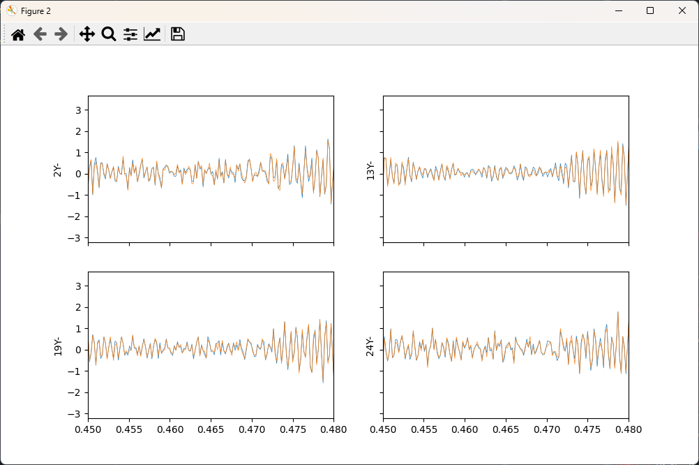
Figure E2.42:Zoom into an impact during the transient control showing good results achieved after the impact.
2.4Summary
This appendix has walked through several example tests using virtual hardware with Rattlesnake. Users are encouraged to use this appendix as a quick-start guide to using Rattlesnake. Rattlesnake constructed equations of motion from a System object from the open-source SDynPy Python package. These equations of motion were integrated over time by Rattlesnake to simulate a test being performed on that structure.
Modal testing was performed using shaker excitation. Modes were fit to the data using the SDynPy Python package. Impact hammer testing could be performed using the combined environments capabilities of Rattlesnake, but that advanced usage would only confuse this beginner-level tutorial, so it was not included in this demonstration.
Vibration testing was performed using simulated modal shakers. A series of impacts was used to create an environment that the vibration test would aim to replicate. Both MIMO Random and MIMO transient vibration tests were run, where the MIMO Random attempted to replicate a prescribed CPSD matrix, and the MIMO Transient attempted to replicate the time history directly. Both control schemes achieved good results.
SDynPy can be installed via pip using
pip install sdynpy, or otherwise downloaded from the Github repository