E3Synthetic Example Problem using State Space Metrics
One final example will be provided which demonstrates the use of State Space matrices to define a virtual system from which a system of equations can be created and integrated. The State Space formulation provides the most flexibility to implement arbitrary systems of equations in Rattlesnake. For example, if the user wanted to substructure a shaker model to a typical mass, stiffness, and damping matrix, this formulation would provide for that flexibility. However, because of this flexibility, it requires a bit more work and care to set up correctly.
In the current example, we will not do anything as complicated as substructuring, but rather construct a state space model from the typical mass, stiffness, and damping matrices directly. However, the user should be aware that state-space models can be used to represent more complex configurations.
3.1Creating a State Space Model
Chapter 8 provides an overview of the State Space Matrices in equations (8.1) and (8.2). They are reproduced here for convenience.
Here is the state matrix, is the input matrix, is the output matrix, is the feedthrough matrix, is the state vector, is the input vector, and is the output vector.
The signals that Rattlesnake outputs are provided to those equations as the inputs to the model, and the signals Rattlesnake measures are the output degrees of freedom . Users must therefore construct the state space matrices , , , and with the correct shape, row order, and column order. The rows of (and therefore the columns of and ) must be in the same order as the excitation rows in the channel table (these will be rows with an entry in the Feedback Device column). Similarly, the rows of (and therefore the rows of and ) must be in the same order as the acquisition rows in the channel table (these will be rows with an entry in the Physical Device column). Note that because Rattlesnake requires its excitation signals to be also measured by the acquisition (e.g., shaker signals must be teed back to acquisition channels for real hardware), there will generally be a row partition of the matrix containing zeros and a row partition of the matrix containing the identity matrix. This would result in the input signals being directly returned as output degrees of freedom . Equation (E3.3) shows this, where a partition of zeros in the matrix and a partition of identity matrix in the matrix results in a partition of the output degrees of freedom being equivalent to the input signals .
3.2Creating the State Space Model
Prior to running virtual control using a state space model, that model must be created along with the channel table corresponding to the output matrices and and the specification that will be controlled.
This example will create a state space model from a beam mass, stiffness, and damping matrix. In this example, we will use SDynPy to generate the beam mass, stiffness, and damping matrices, from which state space matrices will be derived. However, one should note that this is not required. State space matrices can be computed from many different sources. Note that we will use a reduced order model of the system for faster integration. This will require incorporating the reduction transformation that the beam uses.
The first step of this process is to create the beam finite element model. For simplicity, we will use the same code and model used in Example E2.
# Import SDynPy module to get structural dynamics functionality
import sdynpy as sdpy
# We'll also import some common Python packages
import numpy as np # NumPy for numeric calculations
import matplotlib.pyplot as plt # Matplotlib for plotting

# Create a system and geometry object using the beam functionality in SDynPy
system,geometry = sdpy.System.beam(
    length = 24 * 0.0254, # meters
    width = 0.75 * 0.0254, # meters
    height = 1.0 * 0.0254, # meters
    num_nodes = 25,
    material = 'steel')
# We want to see which degrees of freedom we have to work with, so we will
# plot the geometry with coordinate labels
geometry.plot_coordinate(label_dofs=True,arrow_scale=0.02)

# The finite element model system of equations is too large to integrate
# real-time, so we will create a reduced modal system to integrate based on the
# desired bandwidth of the test
test_bandwidth = 2560 # Hz

# Solve for modes up to 1.5x the bandwidth to lessen modal truncation effects
modes = system.eigensolution(maximum_frequency = test_bandwidth*1.5)

# This also gives us the option to add some damping to the model
modes.damping = 0.005

# Transform to modal system: modal mass, modal stiffness, modal damping
modal_system = modes.system()
While SDynPy’s System object has a to_state_space method to automatically construct state space matrices from its internal data, we will instead perform these operations ourselves to demonstrate the approach that can be used if a user is constructing these matrices from some other source. Prior to constructing the state space matrices, we must determine which physical degrees of freedom we wish to use as outputs, and which we wish to use as inputs, as this will determine which rows and columns of the matrices are used. We will use the same degrees of freedom in our channel table as were used in Example E2. These will include Accelerations as response degrees of freedom and Forces as excitation degrees of freedom.
We will first extract the mass matrix , stiffness matrix , damping matrix , and reduction transformation matrix . We will split up the transformation matrix into , which is the rows of corresponding to the physical response degrees of freedom, and , which is the rows of corresponding to the input degrees of freedom. Note that if the system in question is a physical system without any reduction, then the following equations and code still apply, except that the transformation matrix will equal the identity matrix.
# Select degrees of freedom to use in the test, corresponds to the channel table
response_coordinates = sdpy.coordinate_array([2,13,19,24],'Y-')
input_coordinates = sdpy.coordinate_array([2,24],'Y+')

# Extract the System matrices, including transformation matrices.
M = modal_system.M
K = modal_system.K
C = modal_system.C
phi_response = modal_system.transformation_matrix_at_coordinates(response_coordinates)
phi_input = modal_system.transformation_matrix_at_coordinates(input_coordinates)

ndofs = modal_system.ndof
tdofs_response = phi_response.shape[0]
tdofs_input = phi_input.shape[0]
We can then compute the state space matrices from the system matrices.
The state matrix has the equation and code:
A_state = np.block([[np.zeros((ndofs, ndofs)), np.eye(ndofs)],
                    [-np.linalg.solve(M, K), -np.linalg.solve(M, C)]])
The input matrix has the equation and code:
B_state = np.block([[np.zeros((ndofs, tdofs_input))],
                    [np.linalg.solve(M, phi_input.T)]])
Note the inclusion of the transformation matrix which transforms physical inputs into the reduced space so it can be multiplied by the reduced mass matrix .
Our outputs will include accelerations and forces, so we will include those partitions of the output matrix and feedforward matrix . The equations and code are:
C_state = np.block([[-phi_response@np.linalg.solve(M, K), -phi_response@np.linalg.solve(M, C)],
                    [np.zeros((tdofs_input, ndofs)), np.zeros((tdofs_input, ndofs))]])

D_state = np.block([[phi_response @ np.linalg.solve(M, phi_input.T)],
                    [np.eye(tdofs_input)]])
Note the multiplication by the response transformation to transform reduced degrees of freedom to physical degrees of freedom for the output for the top acceleration partition. For the bottom force partition, we have zeros in the matrix and identity in the matrix, so the physical inputs are passed through directly to outputs without any modifications, as required by Rattlesnake. This is the virtual equivalent of teeing the excitation signal into a response channel on a data acquisition system.
We must finally save these matrices to a .mat file or .npz file with fields A, B, C, and D, which can be read by Rattlesnake.
Note that this system is set up with channels in the same order as the channel table shown in Figure E2.27, so we can simply use that channel table for this test. Be aware that the input and response locations are hard-coded into the state space model, therefore if we wish to change the number of shakers or their locations, or change the number of responses or their locations, we must generate a new state space model to use in Rattlesnake. The advantage of the SDynPy approach described in Example E2 is that that hardware will parse the channel table and construct the system equations of motion based off that data, so we need not worry about the channel bookkeeping or generating separate models. While the state space approach offers more flexibility, we must be aware that it is our responsibility to ensure the channel table in Rattlesnake matches the state space system we have created.
np.savez('state_space.npz',A = A_state, B = B_state, C = C_state, D = D_state)3.3Running a Synthetic Vibration Test
Because we have set up our state space system equivalently to the example problem in Example E2, we will utilize the channel table and specifications from that example problem for this example problem as well. Readers are encouraged to fill out a channel table and run the code from that Appendix to generate the specifications if they have not already.
It is worth noting again that attempting to run the Modal test as described in Section 2.2 will not work without modification, because the channel table for that test only utilized one shaker, while our current state space object has two shakers. After completion of this example problem, a good exercise for the reader would be to modify the system object to remove the second shaker, or to add a second shaker to the modal test and run a burst random test with two shakers.
3.3.1Data Acquisition Setup
Now that the state space matrices are constructed, we will set up a random or transient vibration test using the specifications and channel tables developed in Example E2. We will open Rattlesnake and select either the MIMO Random Vibration environment or MIMO Transient Environment.
On the Data Acquisition Setup tab, we will Load Channel Table to import our Excel channel spreadsheet. We will set the Hardware Selector to State Space Integration... and select our state space file state_space.npz, as well as set the sample Sample Rate to 5120. The other parameters can be left at their default values. Figure E3.1 shows these parameters.
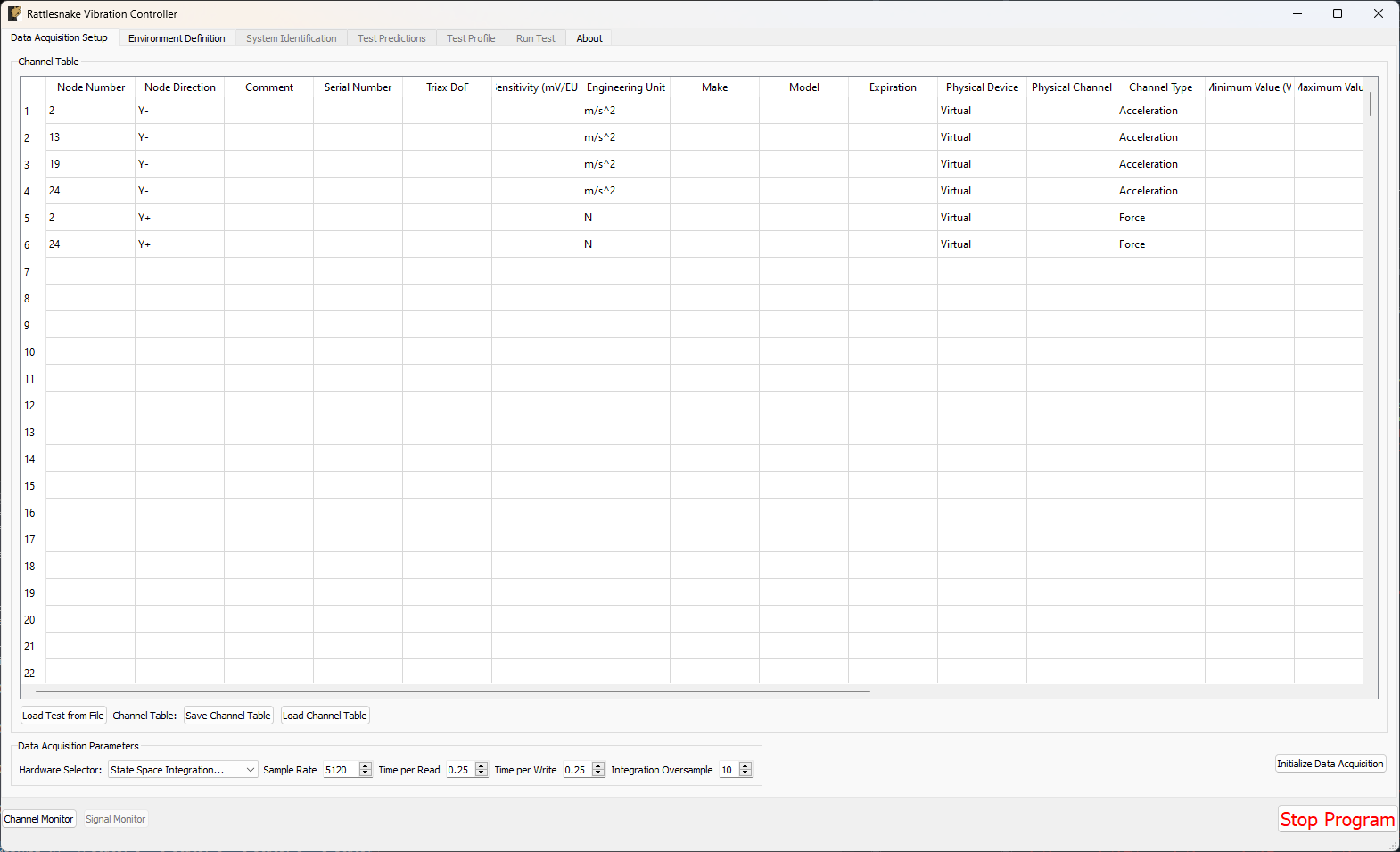
Figure E3.1:Data acquisition setup for the State Space example problem.
Click the Initialize Data Acquisition button to proceed.
3.3.2Environment Setup and Running a Synthetic Test
The remainder of the operations are identical to those described in Section 2.3, so readers are directed to that Section to complete the test. Rattlesnake is designed such that it utilizes largely the same workflow regardless of which data acquisition hardware is being used. Figure E3.2 through Figure E3.5 show screenshots from the Rattlesnake software at different stages of the test. These should look nominally identical to Figure E2.30 through Figure E2.33 from Section 2.3.
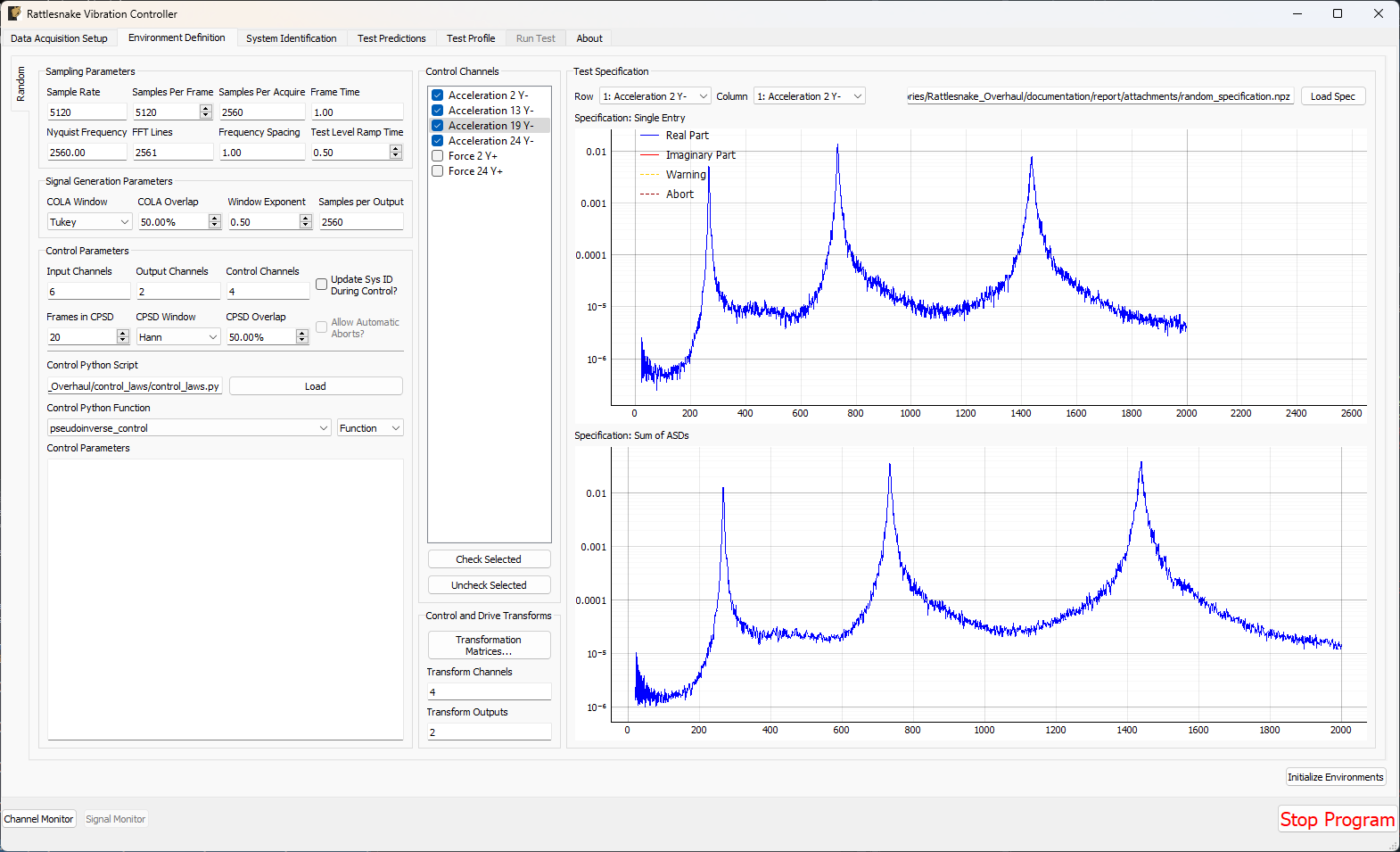
Figure E3.2:Environment Definition for the State Space example problem.
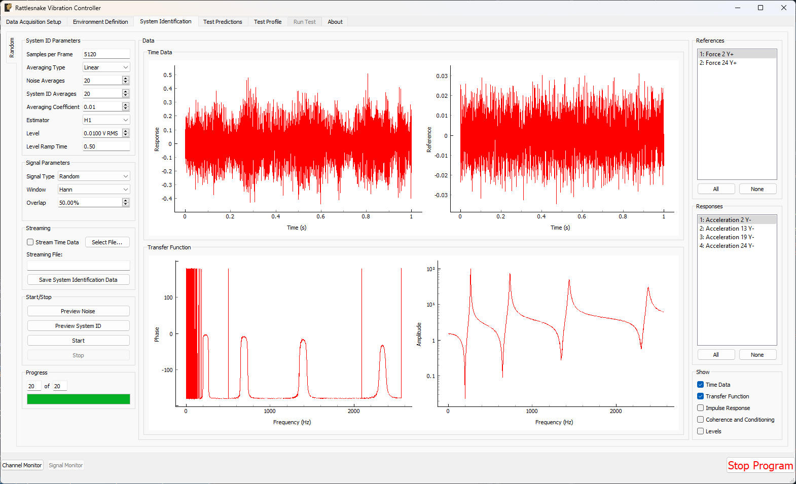
Figure E3.3:System Identification for the State Space example problem
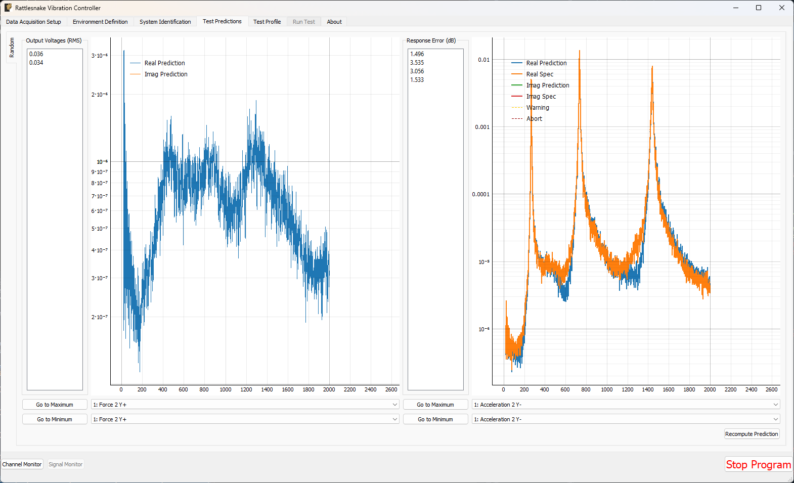
Figure E3.4:Test Predictions for the State Space Example Problem

Figure E3.5:Running a MIMO Random environment with the State Space example problem.
3.4Summary
This appendix has walked through an example test using virtual hardware with Rattlesnake. Users are encouraged to use this Appendix as a quick-start guide to using Rattlesnake. Rattlesnake constructed equations of motion from state space matrices. These equations of motion were integrated over time by Rattlesnake to simulate a test being performed on that structure.
This Appendix only showed the data acquisition setup portion of the controller, as the remaining controller activities are identical to those from Example E2, highlighting Rattlesnake’s common workflow regardless of which data acquistion hardware is used.