Parameter Inference with MCMC

This example (ex_minf_sketch.py) walks through a complete Bayesian parameter inference workflow for a 1-D model using adaptive MCMC. It covers data generation, inference configuration, MCMC sampling, and rich post-processing visualisation.

Source: ex_minf_sketch.py

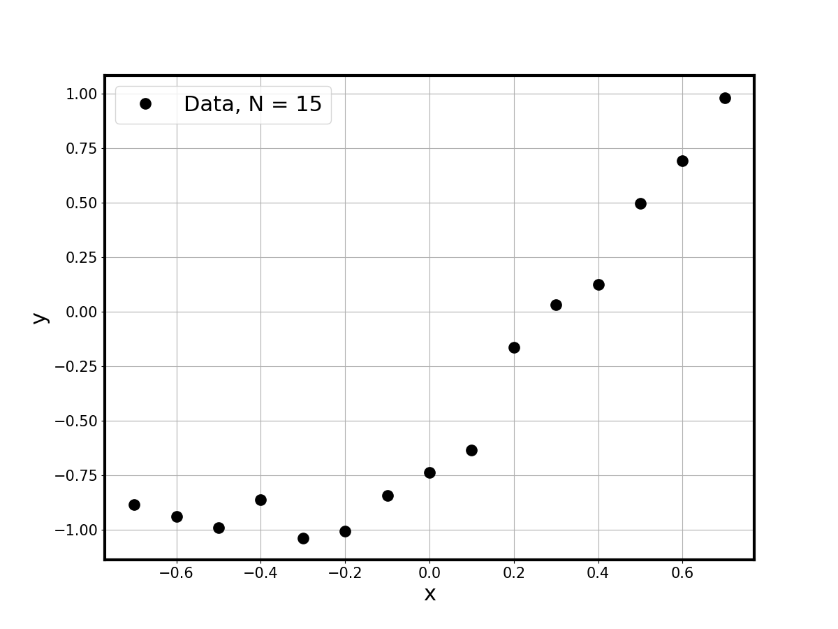
Synthetic Data

A tanh truth model is evaluated on a grid and noisy observations are generated at 15 equally-spaced points:

true_model = tanh_model          # tanh(3*(x - 0.3))
npt = 15
xdata = 0.7 * np.linspace(-1., 1., npt).reshape(-1, 1)
ydata = true_model(xdata) + 0.1 * np.random.randn(npt, 1)

Calibration Model

An exponential model with two parameters is used as the calibration surrogate:

def exp_model_single(par, xx):
    return par[1] * np.exp(par[0] * xx) - 2

The model is deliberately simpler than the truth, so the inference must compensate through its posterior uncertainty.

Inference Configuration

The inference is configured through a single dictionary that controls every aspect of the calibration:

model_infer_config = {
    "inpdf_type" : 'pci',          # PC-based internal PDF
    "pc_type"    : 'LU',           # Legendre-Uniform basis
    "outord"     : 1,              # first-order output PC
    "rndind"     : [0, 1],         # both params are random
    "lik_type"   : 'gausmarg',     # Gaussian marginal likelihood
    "pr_type"    : 'uniform',      # uniform prior (unbounded)
    "dv_type"    : 'var_fixed',    # known data variance
    "dv_params"  : [0.01],         # sigma^2 = 0.1^2
    "calib_type" : 'amcmc',        # adaptive MCMC
    "calib_params": {
        'nmcmc': 10000, 't0': 100,
        'tadapt': 100, 'gamma': 0.1
    },
}

Running MCMC

A single call launches the full inference pipeline — BFGS initialisation followed by adaptive MCMC:

calib_results = minf.model_infer(
    ydata, calib_model, xdata, calib_model_pdim,
    **model_infer_config)

The chain, log-posterior, and acceptance rates are returned in calib_results.

Post-Processing

Posterior model samples are generated by evaluating the calibration model at the MCMC chain points and collecting predictive statistics:

checkmode = [calib_results['post'].model, xgrid,
             range(len(xgrid)), md_transform]
ycheck_pred, samples = minf.model_infer_postp(
    calib_results, checkmode=checkmode,
    nburn=len(calib_results['chain']) // 10,
    nevery=10, nxi=1)

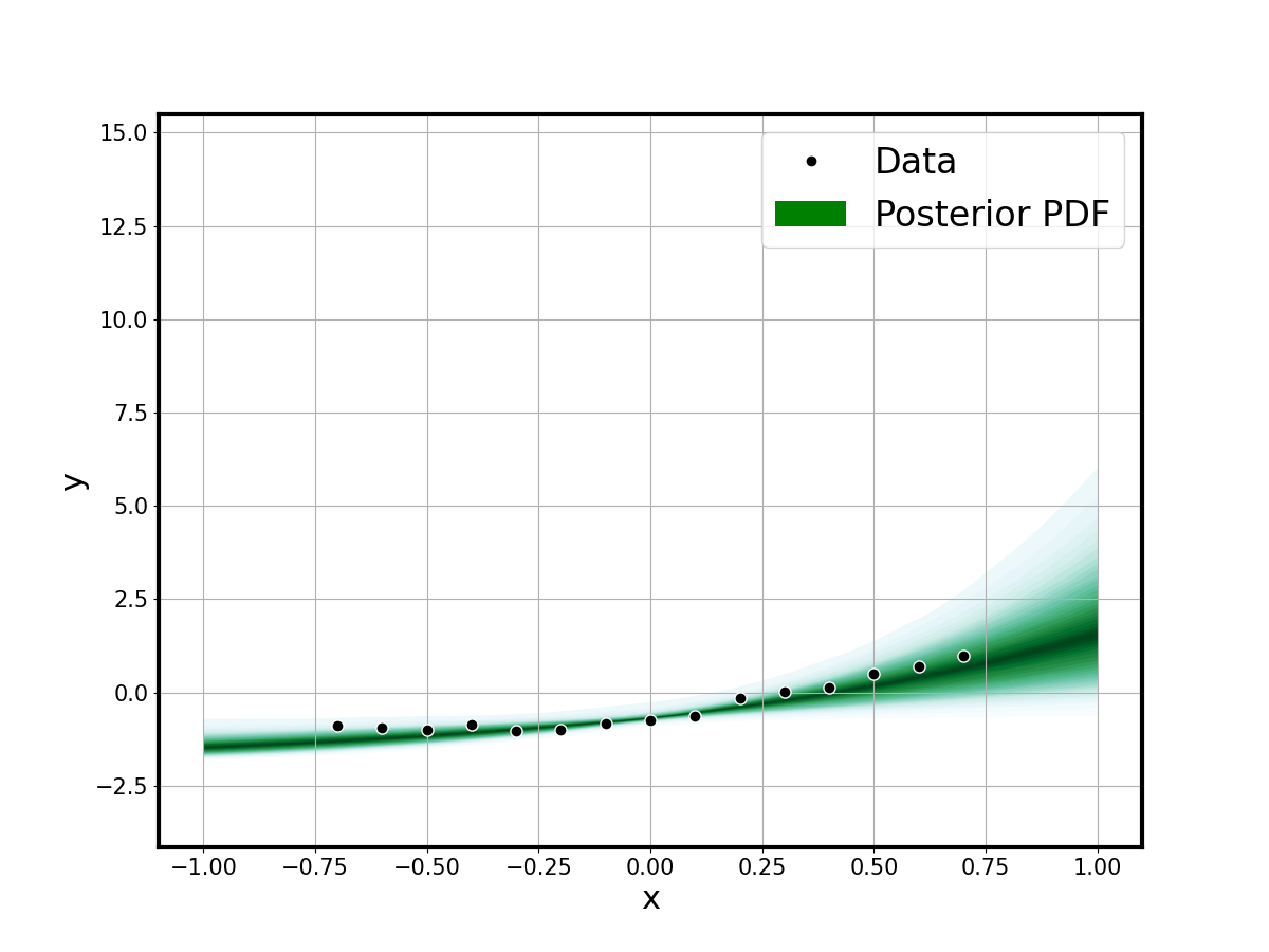
Predictive Fit

The shaded predictive envelope shows the calibrated model uncertainty against data and the true model:

fsamples_2d = np.reshape(samples['fmcmc'], (-1, ngrid), order='F')
minf.plot_1dfit_shade(xgrid, fsamples_2d.T, xydata=(xdata, ydata))

A parity plot compares the true model output per grid point with the calibrated posterior mean:

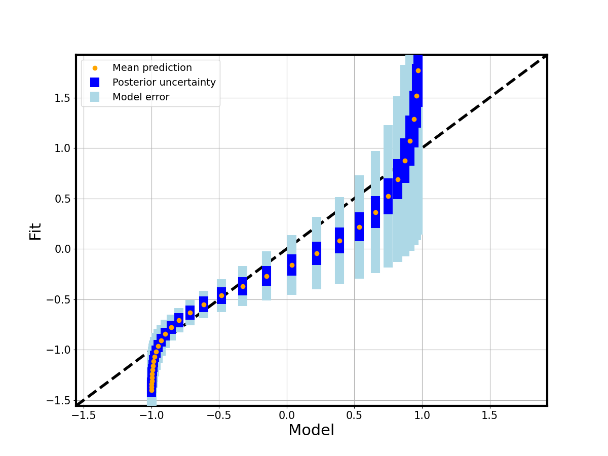
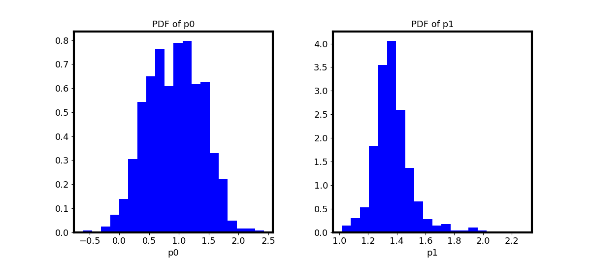
Parameter Posteriors

Marginal and joint posterior distributions of the two exponential-model parameters are visualised:

pl.plot_pdfs(samples_=psamples_2d, plot_type='inds')