Bayesian Compressive Sensing for Sparse PC Regression
This example (ex_bcs.py) demonstrates how to use Bayesian Compressive
Sensing (BCS) to construct a sparse polynomial chaos (PC) surrogate model.
BCS automatically identifies the most relevant basis terms, yielding a
compact representation of the target function.
Source: ex_bcs.py
Setup
The example creates synthetic 2-d data from a test function with added noise:
N = 144          # number of samples
dim = 2          # input dimensionality
order = 5        # maximum polynomial order
datastd = 0.01   # noise standard deviation

true_model = fcb.prodabs   # target function |x1*x2|

domain = np.ones((dim, 2)) * np.array([-1., 1.])
x = scale01ToDom(np.random.rand(N, dim), domain)
y = true_model(x) + datastd * np.random.randn(N)
Build the PC Basis
A full-tensor multiindex of order 5 in 2 dimensions is created (21 terms).
The PC basis matrix Amat is then evaluated at the sample points:
mindex = get_mi(order, dim)         # 21-term multiindex
pcrv = PCRV(1, dim, 'LU', mi=mindex)
Amat = pcrv.evalBases(x, 0)        # (144, 21) design matrix
BCS Fit
BCS is run with tolerance eta=1e-11 to select the most relevant basis
terms. The smaller eta is, the more terms BCS retains:
lreg = bcs(eta=1.e-11)
lreg.fita(Amat, y)
After fitting, lreg.used contains the indices of the surviving basis
terms and lreg.cf holds their coefficients. For the prodabs
function the dominant terms are the even-powered ones (0,0), (2,0),
(0,2), (2,2), (4,0), (0,4), which matches the symmetry
of \(|x_1 x_2|\).
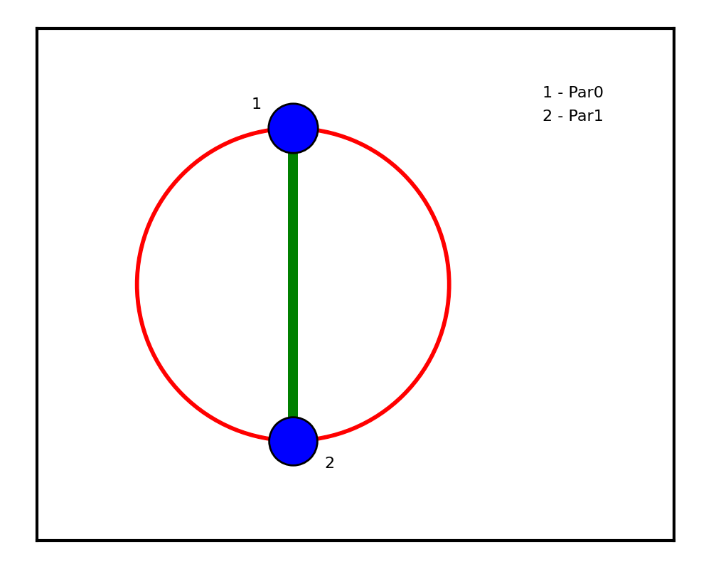
Sensitivity Analysis
Total and joint Sobol sensitivities are computed analytically from the sparse PC coefficients:
pcrv.setMiCfs([mindex[lreg.used, :]], [lreg.cf])
mainsens = pcrv.computeTotSens()
jointsens = pcrv.computeJointSens()
plot_jsens(mainsens[0], jointsens[0])
The resulting sensitivity pie chart shows that both inputs contribute roughly equally (~57 % and ~56 %), with a non-trivial joint sensitivity (~14 %) reflecting the \(|x_1 x_2|\) coupling.
Parity Plot
A diagonal (parity) plot compares the true function values with the BCS surrogate predictions, including error bars from the predictive variance:
yy_pred, yy_pred_var, _ = lreg.predicta(Amat[:, lreg.used], msc=1)
plot_dm([y], [yy_pred],
        errorbars=[[np.sqrt(yy_pred_var), np.sqrt(yy_pred_var)]],
        labels=['Training'], colors=['b'],
        axes_labels=['Model', 'Poly'],
        figname='fitdiag.png')
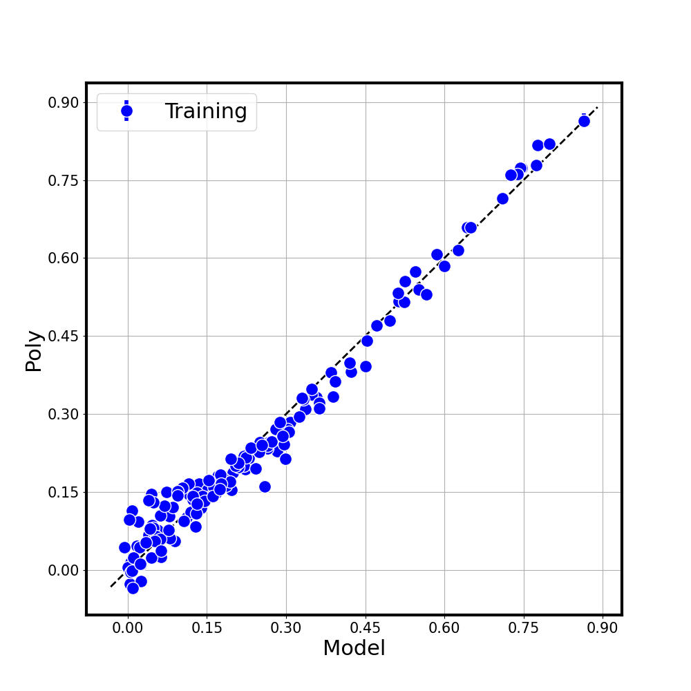
Points clustering tightly around the diagonal indicate a good fit.
Console Output
Typical console output (truncated) for the default settings:
Full multiindex basis:
[[0 0] [1 0] [0 1] ... [0 5]]

Indices of survived bases:
[ 0  3  5 12 10 14  1  4 18  7 20  9 13  8  2 11  6 15]

Reduced multiindex and corresponding coefficients
[0 0]  0.253
[2 0]  0.323
[0 2]  0.317
[2 2]  0.404
[4 0] -0.089
[0 4] -0.094
...

Main Sensitivities:   [0.575 0.560]
Joint Sensitivities:  [[0.    0.135]
                       [0.135 0.   ]]