Simulating Shaker Effects in SDynPy - SDynPy: A Structural Dynamics Python Package

This page demonstrates how we can add shaker effects to a SDynPy system.

import sdynpy as sdpy
import numpy as np

Shaker Modeling¶

Vibration shakers are electro-mechanical systems that transform electrical inputs (typically voltage, though other amplifier modes exist) into a mechanical excitation of a structure. SDynPy uses a system of equations with four degrees of freedom. The mechanical portion of the shaker itself is split into three portions: the shaker body, the shaker armature, and the shaker attachment point to the structure; each of these have one degree of freedom of motion. The fourth degree of freedom is the current in the shaker armature, which is an electrical quantity. Inputs to this system can be forces at any of the three mechanical degrees of freedom or a prescribed voltage. This modeling is based on the paper by G.F. Lang in the Sound and Vibration Magazine titled “Electrodynamic Shaker Fundamentals.” A schematic of this model is shown in the following figure, which is taken from R. Schultz’s paper “Calibration of Shaker Electro-Mechanical Models” which was presented at the 2020 International Modal Analysis Conference.

The equations of motion for this system is

\mathbf{M}_{shk} = \begin{bmatrix} M_1 & 0 & 0 & 0 \\ 0 & M_2 & 0 & 0 \\ 0 & 0 & M_3 & 0 \\ 0 & 0 & 0 & 0\end{bmatrix}

(1)

\mathbf{C}_{shk} = \begin{bmatrix} C_{12}+C_{13} & -C_{12} & -C_{13} & 0 \\ -C_{12} & C_{12} & 0 & 0 \\ -C_{13} & 0 & C_{13} & 0 \\ BL & -BL & 0 & L_e\end{bmatrix}

(2)

\mathbf{K}_{shk} = \begin{bmatrix} K_{12}+K_{13} & -K_{12} & -K_{13} & -BL \\ -K_{12} & K_{12} & 0 & BL \\ -K_{13} & 0 & K_{13} & 0 \\ 0 & 0 & 0 & R_e\end{bmatrix}

(3)

\mathbf{M}_{shk}\begin{bmatrix}\ddot{x}_1 \\ \ddot{x}_2 \\ \ddot{x}_3 \\ \ddot{i}\end{bmatrix} + \mathbf{C}_{shk}\begin{bmatrix}\dot{x}_1 \\ \dot{x}_2 \\ \dot{x}_3 \\ \dot{i}\end{bmatrix} + \mathbf{K}_{shk}\begin{bmatrix}{x}_1 \\ {x}_2 \\ {x}_3 \\ {i}\end{bmatrix} = \begin{bmatrix}{f}_1 \\ {f}_2 \\ {f}_3 \\ {e}\end{bmatrix}

(4)

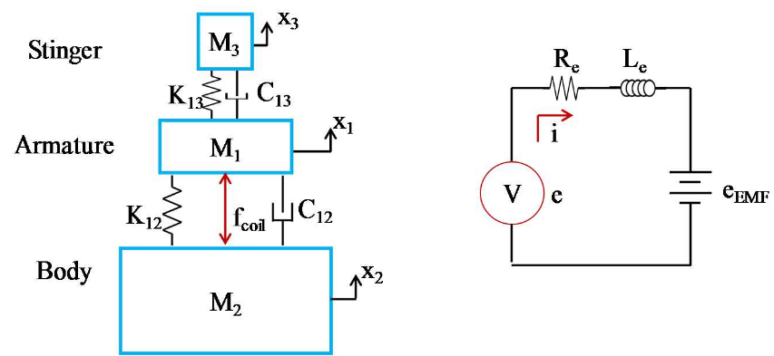
In the above equations, $M_1$ is the armature mass, $M_2$ is the body mass, $M_3$ is the stinger, force gauge, or shaker table mass, $K_{12}$ is the stiffness of the spring between the armature and body, $C_{12}$ is the damping of the spring between the armature and body, $K_{13}$ is the stiffness of the stinger or shaker table attachment, $C_{13}$ is the damping of the stinger or shaker table attachment. The electrical model consists of a resistor with resistance $R_e$ and an inductor with inductance $L_e$ . A voltage source $e$ introduces current in the wire $i$ . Forces $f_1$ , $f_2$ , and $f_3$ could be applied, but these are generally zero as the shaker is generally excited electrically.

Coupling between the electrical model and mechanical model is represented in the model by the force factor $BL$ , which produces a force $f_{coil}$ on the mechanical shaker structure due to the current in the electric circuit. Similarly, motion of the shaker produces a back electromotive force $e_{EMF}$ on the electric circuit.

One additional quantity of interest that a user may desire is the force applied to the structure by the shaker. This can be extracted from the stinger forces as

f_{stinger} = K_{13}(x_1-x_3) + C_{13}(\dot{x}_1-\dot{x}_3)

(5)

Creating Shakers in SDynPy¶

The SDynPy class sdpy.shaker.Shaker4DoF represents shaker models of this form. Inputs to this class are calibrated parameters representing different shakers. This class has class methods representing specific shaker types, allowing users to easily store and pull calibrated parameters. For example, the parameters calibrated from a Modal Shop 100 pound modal shaker in R. Schultz’s paper “Calibration of Shaker Electro-Mechanical Models” are stored in Shaker4DoF.modal_shop_100lbf.

# Create the shaker manually
shaker = sdpy.shaker.Shaker4DoF(m_armature=0.44,
                                m_body=15,
                                m_forcegauge=1e-2,
                                k_suspension=1.1e5,
                                k_stinger=9.63e6,
                                c_suspension=9.6,
                                c_stinger=0.42,
                                resistance=4,
                                inductance=6e-4,
                                force_factor=36)
# Or pull from a stored classmethod
shaker = sdpy.shaker.Shaker4DoF.modal_shop_100lbf()

Obviously, shakers are not terribly interesting unless they are connected to some structure of interest that we wish to simulate. In this case, we will pull out the plate structure from sdynpy.demo.

from sdynpy.demo.beam_plate import system,geometry

This initial system is not very realistic due to lack of damping, and is also somewhat expensive to run as a full physical system, so we will convert it to a modal system and add damping.

modes = system.eigensolution(num_modes=100) # Solve for modes
modes.damping = 0.01 # Add damping
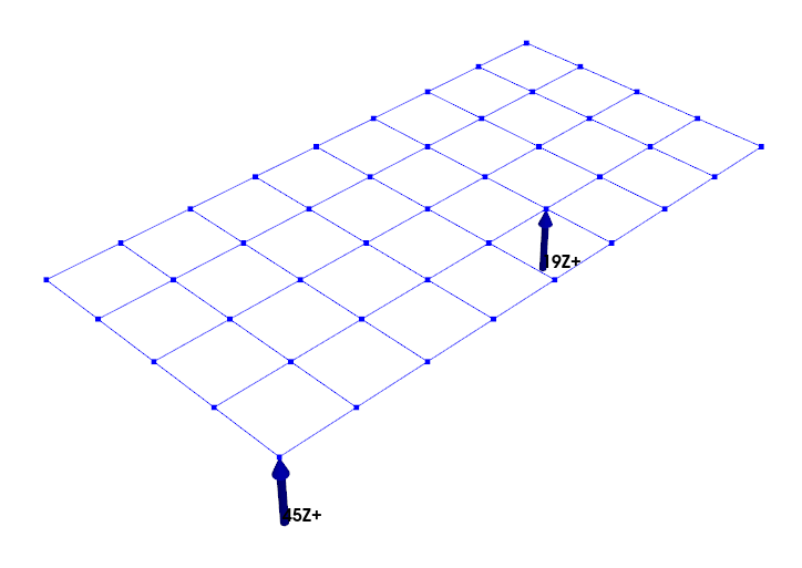
system = modes.system() # Create a modal system from the modes

For this work, we will measure responses at all vertical degrees of freedom, and put our shakers at nodes 45 and 19 in the vertical direction.

responses = sdpy.coordinate_array(geometry.node.id,'Z+')
drive_points = sdpy.coordinate_array([45,19],'Z+')

geometry.plot_coordinate(responses,label_dofs=True)
geometry.plot_coordinate(drive_points,label_dofs=True, arrow_ends_on_node=True);

<sdynpy.core.sdynpy_geometry.GeometryPlotter at 0x1c53f4fa4e0>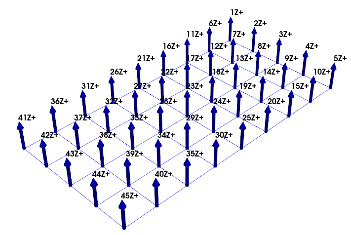

For simplicity, we will simply use two of the Modal Shop 100 lbf shakers at these drive locations.

shaker_1 = sdpy.shaker.Shaker4DoF.modal_shop_100lbf()
shaker_2 = sdpy.shaker.Shaker4DoF.modal_shop_100lbf()

Now, we need to attach our shakers to our structure. While we could go through the substructuring calculations to constrain the force gauge from the shaker models to connect to the prescribed drive point locations of the structure, we will instead use a convenient method that exists in SDynPy called substructure_shakers. This method takes as its inputs the shaker models to attach to the structure and the drive point locations at which the shakers will be attached. It handles all of the bookkeeping behind the scenes to attach the shakers to the structure. As with all substructuring functions in SDynPy, it doesn’t matter if the System we are attaching to is a physical system or a reduced system (e.g. a modal or Craig-Bampton system), since SDynPy will handle the reduction transformation seamlessly. In our present case, we have a modal system, yet we can proceed as usual without any special considerations.

system_w_shakers = system.substructure_shakers(
    [shaker_1, shaker_2], # The two shakers to attach
    drive_points) # The two coordinates to attach the shakers

When we perform substructure_shakers, SDynPy will go through and assign degree of freedom labels to the shaker degrees of freedom similar to the above equations of motion. SDynPy will first find the maximum node identification number in the System object to which the shakers are being attached. It will then find the next highest power of ten as a starting node for the shakers. E.g. if the highest node number in the system is 58, then the shaker degrees of freedom will be in the 100s, since 100 is the next power of 10 greater than 58.

The 10s place in the node numbers refer to the shaker number. The first shaker will have nodes with a 0 in the 10s place, the second will have nodes with a 1 in the 10s place, and so on. The ones place will be one of 1, 2, 3, or 4, representing the degrees of freedom in the above shaker equations of motion. Degrees of freedom 1, 2, and 3, representing mechanical degrees of freedom, simply have a direction of ‘X+’ assigned to them. The electrical degree of freedom is directionless. Let’s look at the last 10 degrees of freedom in our system.

system_w_shakers.coordinate[-10:]

coordinate_array(string_array=
array(['45RY+', '45RZ+', '101X+', '102X+', '103X+', '104', '111X+',
       '112X+', '113X+', '114'], dtype='<U5'))

Here we can see the last “physical” degrees of freedom in our system have node number 45, meaning that shaker degrees of freedom will start with node 100, which is the next largest power of 10. Then we have two shakers represented by node numbers in the 100s and 110s, respectively. For example, degree of freedom 113X+ represents the second shaker (1 in the 10s place) and the third degree of freedom (3 in the 1s place), which is the motion of the force gauge.

The excitation voltages to the shakers are then the degrees of freedom greater than 100 that end in 4.

input_coordinates = sdpy.coordinate_array([104,114],'') # '' means no direction associated with voltage

Massless Degrees of Freedom and Transforming to State Space¶

To integrate equations of motion, we will generally transform the system of equations to state space, which can then be integrated over time. However, one challenging aspect of the present system is the lack of an equivalent mass term for certain degrees of freedom. The typical transformation between the second-order equations of motion and the first-order state space equations involves inverting the mass matrix. However, we see that an entire row of the mass matrix corresponding to the electrical degree of freedom in the shaker model is zero. Therefore, we cannot simply invert this matrix. Instead we must separate the equations of motion into massless and massive degrees of freedom and transform to states space separately.

The equations presented below assume a physical system, but can be generalized to a reduced system by including transformation matrix terms.

We will split up the general second-order differential equation of motion into degrees of freedom containing mass, and those not containing mass. We will denote the massive degrees of freedom with subscript 1 and massless degrees of freedom with subscript 2. The system matrices will then be split up into superscripts 11, 12, 21, and 22 corresponding to different combinations of massless and massive degrees of freedom.

\begin{bmatrix}\mathbf{M}_{11} & \mathbf{0} \\ \mathbf{0} & \mathbf{0} \end{bmatrix}\begin{bmatrix}\ddot{\mathbf{x}}_1 \\ \ddot{\mathbf{x}}_2\end{bmatrix} + \begin{bmatrix}\mathbf{C}_{11} & \mathbf{C}_{12} \\ \mathbf{C}_{21} & \mathbf{C}_{22} \end{bmatrix}\begin{bmatrix}\dot{\mathbf{x}}_1 \\ \dot{\mathbf{x}}_2\end{bmatrix} + \begin{bmatrix}\mathbf{K}_{11} & \mathbf{K}_{12} \\ \mathbf{K}_{21} & \mathbf{K}_{22} \end{bmatrix}\begin{bmatrix}{\mathbf{x}}_1 \\ {\mathbf{x}}_2\end{bmatrix} = \begin{bmatrix}\mathbf{f}_1 \\ \mathbf{f}_2\end{bmatrix}

(6)

We can split these matrix equations into two separate equations.

\mathbf{M}_{11}\ddot{\mathbf{x}}_1 + \mathbf{C}_{11}\dot{\mathbf{x}}_1 + \mathbf{C}_{12}\dot{\mathbf{x}}_2 + \mathbf{K}_{11}\mathbf{x}_1 + \mathbf{K}_{12}\mathbf{x}_2 = \mathbf{f}_1

(7)

\mathbf{C}_{21}\dot{\mathbf{x}}_1 + \mathbf{C}_{22}\dot{\mathbf{x}}_2 + \mathbf{K}_{21}\mathbf{x}_1 + \mathbf{K}_{22}\mathbf{x}_2 = \mathbf{f}_2

(8)

The typical state space transformation consists of replacing the double derivatives with a single derivative using a substitution $\dot{\mathbf{x}}_1 = \mathbf{v}_1$ :

\mathbf{M}_{11}\dot{\mathbf{v}}_1 + \mathbf{C}_{11}{\mathbf{v}}_1 + \mathbf{C}_{12}\dot{\mathbf{x}}_2 + \mathbf{K}_{11}\mathbf{x}_1 + \mathbf{K}_{12}\mathbf{x}_2 = \mathbf{f}_1

(9)

\mathbf{C}_{21}{\mathbf{v}}_1 + \mathbf{C}_{22}\dot{\mathbf{x}}_2 + \mathbf{K}_{21}\mathbf{x}_1 + \mathbf{K}_{22}\mathbf{x}_2 = \mathbf{f}_2

(10)

This leaves us with the states $\mathbf{x}_1$ , $\mathbf{v}_1$ , and $\mathbf{x}_2$ . We typically would like to solve the state derivatives $\dot{\mathbf{x}}_1$ , $\dot{\mathbf{v}}_1$ , and $\dot{\mathbf{x}}_2$ , so we should solve for those equations. We already have an equation for $\dot{\mathbf{x}}_1$ from the substitution:

\dot{\mathbf{x}}_1 = \mathbf{v}_1

(11)

We can solve for $\dot{\mathbf{x}}_2$ from the second of the two partitioned equations:

\dot{\mathbf{x}}_2 = -\mathbf{C}_{22}^{-1}\mathbf{C}_{21}\mathbf{v}_1 + \mathbf{C}_{22}^{-1}\mathbf{f}_2 - \mathbf{C}_{22}^{-1}\mathbf{K}_{21}\mathbf{x}_1 - \mathbf{C}_{22}^{-1}\mathbf{K}_{22}\mathbf{x}_2

(12)

We can substitute the equation for $\dot{\mathbf{x}}_2$ into the first of the partitioned equations to solve for $\dot{\mathbf{v}}_1$ :

\dot{\mathbf{v}}_1 = -\mathbf{M}_{11}^{-1}\mathbf{C}_{11}\mathbf{v}_1 + \mathbf{M}_{11}^{-1}\mathbf{C}_{12}\mathbf{C}_{22}^{-1}\mathbf{C}_{21}\mathbf{v}_1 + \mathbf{M}_{11}^{-1}\mathbf{C}_{12}\mathbf{C}_{22}^{-1}\mathbf{K}_{21}\mathbf{x}_1 + \mathbf{M}_{11}^{-1}\mathbf{C}_{12}\mathbf{C}_{22}^{-1}\mathbf{K}_{22}\mathbf{x}_2 - \mathbf{M}_{11}^{-1}\mathbf{C}_{12}\mathbf{C}_{22}^{-1}\mathbf{f}_2 - \mathbf{M}_{11}^{-1}\mathbf{K}_{11}\mathbf{x}_1 - \mathbf{M}_{11}^{-1}\mathbf{K}_{12}\mathbf{x}_2 + \mathbf{M}_{11}^{-1}\mathbf{f}_1

(13)

We can then extract coefficients of each of the state terms and inputs to assemble the state space matrices. Note that SDynPy will handle all of these calculations behind the scenes, so we don’t have to think too hard about them. However, it will be important to know how SDynPy handles these degrees of freedom internally so we can assemble extra output degrees of freedom based on these terms. Particularly it is important to know that SDynPy partitions out the massless degrees of freedom and handles them separately from the massive degrees of freedom.

Extra Output Degrees of Freedom¶

Users of SDynPy system objects will be familiar with its time integration capabilities. Users can generally provide the degrees of freedom desired in the form of a CoordinateArray, and SDynPy will automatically select the correct rows and columns of the matrices to use in its calculations. However, sometimes there are quantities of interest that are not always directly available in the objects. For example, the force applied to the structure via the shaker is generally of interest, and this is computed by relative displacements and velocities scaled by stiffness and damping values.

f_{stinger} = K_{13}(x_1-x_3) + C_{13}(\dot{x}_1-\dot{x}_3)

(14)

SDynPy allows us to pass extra_outputs to its time integration functions, allowing us to append output degrees of freedom to the time integration. However, we must construct these extra outputs as we would the $C$ and $D$ state space matrices. Therefore we need to know how SDynPy sorts its degrees of freedom in the state space form. This is shown in the to_state_space documentation, but is repeated here for clarity.

SDynPy sorts its states first as massive displacements $\mathbf{x}_1$ , then massive velocities $\mathbf{v}_1$ , then massless displacements $\mathbf{x}_2$ . To construct the stinger forces, we only need to deal with massive degrees of freedom, so we can let the massless state coefficients be zero here.

Let’s manipulate the equation for the force at the stinger, transforming it to a general equation that would also accept reduced order systems (which will be key, because our current system is a reduced order system, both from the modal transformation and subsequent substructuring calculation).

In the case of a general reduced order system, the degrees of freedom $\mathbf{x}_1$ and velocities $\mathbf{v}_1$ are not physical degrees of freedom, but some reduced degrees of freedom. We transform from these reduced degrees of freedom to the physical degrees of freedom via the reduction transformation $\mathbf{\Phi}$ . We can, of course, partition the rows of $\mathbf{\Phi}$ to give us the physical values of interest. For example to recover the first degree of freedom, we would take the first row of $\mathbf{\Phi}$ and multiply it by all of the states $\mathbf{\Phi}_1\mathbf{x}$ . We could imagine the situation of a physical system, where the transformation $\mathbf{\Phi}$ is the identity matrix, in which case the first row of the identity matrix would pick off the first entry in $\mathbf{x}$ , giving us the first physical degree of freedom.

We can then rewrite the equation as

f_{stinger} = K_{13}(\mathbf{\Phi}_{armature}\mathbf{x}_1-\mathbf{\Phi}_{forcegauge}\mathbf{x}_1) + C_{13}(\mathbf{\Phi}_{armature}\mathbf{v}_1-\mathbf{\Phi}_{forcegauge}\mathbf{v}_1)

(15)

Bringing it into the state space form, we can write it as

f_{stinger} = \begin{bmatrix}K_{13}(\mathbf{\Phi}_{armature}-\mathbf{\Phi}_{forcegauge}) & C_{13}(\mathbf{\Phi}_{armature}-\mathbf{\Phi}_{forcegauge}) & \mathbf{0} \end{bmatrix}\begin{bmatrix}\mathbf{x}_1 \\ \mathbf{v}_1 \\ \mathbf{x}_2\end{bmatrix} + [\mathbf{0}][\mathbf{u}]

(16)

The $C$ matrix is the matrix multiplying the states and the $D$ matrix (here zeros) is multiplying the inputs $\mathbf{u}$ . We can construct this in SDynPy making sure the values are the correct sizes, and ensuring we are only looking at the massive degrees of freedom. We eventually put these matrices into a dictionary along with the coordinate names to assign these output degrees of freedom to pass as an argument to the time integration functions.

massless_dofs = system_w_shakers.massless_dofs # Find the dofs associated with electrical quantities so we can exclude them

# Extract transformation matrices at the armature and force gauge
Phi_arm = system_w_shakers.transformation_matrix_at_coordinates(sdpy.coordinate_array([101,111],1))[:,~massless_dofs]
Phi_fg = system_w_shakers.transformation_matrix_at_coordinates(sdpy.coordinate_array([103,113],1))[:,~massless_dofs]

# Put together the stinger stiffnesses and dampings from our shaker models in a broadcastable form
stinger_stiffnesses = np.array([shaker_1.k_stinger,
                                shaker_2.k_stinger])
stinger_dampings = np.array([shaker_1.c_stinger,
                            shaker_2.c_stinger])

# Create the zeros matrix with the right size
Zml = np.zeros([Phi_arm.shape[0],massless_dofs.sum()])

# Assemble the matrices and put them into a dictionary describing the degrees of freedom.
C = np.concatenate([stinger_stiffnesses[:,np.newaxis]*(Phi_arm-Phi_fg), stinger_dampings[:,np.newaxis]*(Phi_arm-Phi_fg), Zml],axis=1)
D = np.zeros((2,2))

extra_outputs = {'coordinate':drive_points, # Give them the same name as the drive points.
                 'C':C,
                 'D':D}

Simulating a Test and Comparing Results¶

Now that we have our system objects from the substructuring and the extra outputs to get the stinger forces, we can simulate a test. We could use the time_integrate method with any arbitrary force, but for simplicity here, we will simply use the simulate_test method, which will allow us to quickly get data out that we can investigate. We will run a burst random test by applying voltages to our shakers attached to our plate system. We must therefore specify these as the inputs. Also, we must specify which degrees of freedom we want as outputs. SDynPy allows us to select if we want displacement, velocity, or acceleration quantities by supplying a dictionary where the key is the displacement derivative (0 - displacement, 1 - velocity, 2 - acceleration) and the value is the degrees of freedom with that derivative. For example, we may want the current out (a displacement quantity rather than one of its time derivatives) while also desiring the accelerations out.

response_coordinates = {2:responses,0:input_coordinates} # Gives responses from the geometry and the drive current

We can then simulate the test.

response_shaker,reference_shaker = system_w_shakers.simulate_test(
    4000,8000,5,'burst random',input_coordinates,response_coordinates,
    integration_oversample = 5, extra_outputs = extra_outputs)

One good comparison to make is to check if computing FRFs from these time signals gives us the same FRFs as inverting the system matrices.

# Compute FRFs from time histories
frf_shaker = sdpy.TransferFunctionArray.from_time_data(reference_shaker,response_shaker,8000)
# Compute FRFs directly from system matrices
f = np.unique(frf_shaker.abscissa)[1::10] # Get rid of zero frequency and use only a handful of frequencies to speed up computations
frf_shaker_direct = system_w_shakers.frequency_response(f,responses,input_coordinates,displacement_derivative=2)
# Plot to compare
gp_shaker = sdpy.GUIPlot(Direct=frf_shaker_direct, Time_Integrate=frf_shaker[frf_shaker_direct.coordinate])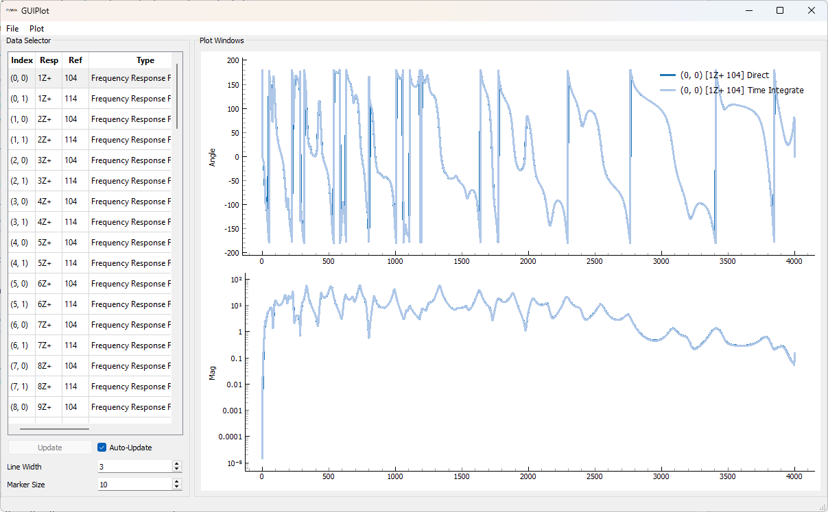

The above calculations used the voltages as the references; however for a typical modal test, we would generally expect to use forces as a reference, so let’s check those results. We can pull off the forces given to use as an extra output as the last two channels of the response time history.

# Last two responses are stinger forces, the rest are the acceleration responses
frf_shaker_force = sdpy.TransferFunctionArray.from_time_data(response_shaker[-2:],response_shaker[:-2],8000)

To show that these were accurately reproduced, we can compare the force-to-response FRFs to the same FRFs computed from the original system before any shakers were attached to it. In this case, the inputs to the system are forces, so we can directly compare the force-to-response FRFs from the bare system to those from the system with shakers attached, which should produce identical results (excepting the small additional mass added to the system by the force gauge, which causes frequencies to drop slightly).

# Set up integration with the original system, not system_w_shakers
response_coordinates_bare = {2:responses}
response_bare,reference_bare = system.simulate_test(4000,8000,5,'burst random',drive_points,response_coordinates_bare,
                                                    integration_oversample = 5)
frf_bare = sdpy.TransferFunctionArray.from_time_data(reference_bare, response_bare,8000)
# Plot the results
gp_bare = sdpy.GUIPlot(Bare_System=frf_bare,
                       From_Shaker_Stinger_Force = frf_shaker_force[frf_bare.coordinate])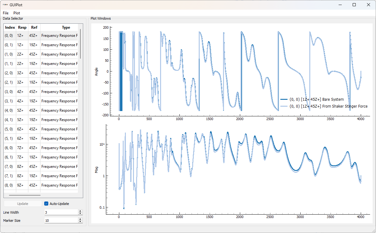

Summary¶

SDynPy makes it easy to simulate shaker effects on your test by allowing you to easily substructure shaker models to your system with substructure_shakers. We can then easily apply voltages to the shakers and integrate equations of motion or compute frequency response. SDynPy gives use the flexibility to request non-standard outputs such as the shaker forces by adding additional rows to the $C$ and $D$ matrices in the state space formulation, giving a good amount of flexibility for users to output precisely the values they care about.