Regression testing for sansmic#
This Jupyter Notebook provides regression testing for sansmic. The results of a the “baseline.dat” input file are stored in a JSON formatted file in this directory (“baseline.json”) and in the “baseline.tst” file directly output from the SANSMIC V02.02 code. Version (V02.02) contains two minor changes by @dbhart: (a) fixed incorrect value for the conversion of barrels to cubic feet that has been present in the V02.01 code since at least 2014, and more likely since at least 1991, and (b) change the output to be based on the number of steps rather than the error-accumulating TIMET variable. Aside from the fix of the conversion factor, the internals of the FORTRAN have remained unmodified since it was validated by Weber, Lord, and Rudeen.
This notebook compares the outputs of sansmic>=1.0.0 to the outputs of SANSMIC==02.02.2024.
Initialize and load the baseline configuration#
[1]:
import sansmic
import numpy as np
import matplotlib.pylab as plt

model = sansmic.io.read_scenario("baseline.dat")
tstF = sansmic.io.read_tst_file("baseline.tst.txt")
resF = sansmic.io.read_json_results("baseline.json")
Note that there are three warnings regarding the cavern specific gravity. A discrepancy between the old documentation and the actual code was discovered while preparing the new sansmic-1.0 package; documentation states that the “REPEAT” option would keep the final concentration of the specific gravity from the previous stage – it did not. The actual switch was for the cavern sg to be set to 1.0 or less. The behavior of the scenario reader is to respect what is in the documentation, not what appears to have been a bug.
To check the scenario reader, write the model to a new-style TOML-formatted file and then read it back in and print it.
[2]:
# Write the new-style config file and print it back out
new_config = "regression.toml"
sansmic.io.write_scenario(model, new_config)
with open(new_config, "r") as fin:
    for line in fin.readlines():
        print(line.strip())
title = 'Converted from DAT-file'
comments = """
Conversion report:
* Floor depth was 4000. ft MD; all heights converted to MD using this value.
"""
num-cells = 100
geometry-data.radii = [10.0, 75.0, 100.0, 100.0, 100.0, 100.0, 100.0, 100.0, 100.0, 100.0, 100.0, 100.0, 100.0, 100.0, 100.0, 100.0, 100.0, 100.0, 100.0, 100.0, 100.0, 100.0, 100.0, 100.0, 100.0, 100.0, 100.0, 100.0, 100.0, 100.0, 100.0, 88.0, 88.0, 88.0, 88.0, 88.0, 88.0, 88.0, 88.0, 88.0, 88.0, 88.0, 88.0, 88.0, 88.0, 88.0, 88.0, 88.0, 88.0, 88.0, 75.0, 75.0, 75.0, 75.0, 75.0, 75.0, 75.0, 75.0, 75.0, 75.0, 75.0, 75.0, 75.0, 75.0, 75.0, 75.0, 75.0, 75.0, 75.0, 75.0, 75.0, 50.0, 35.0, 10.0, 2.0, 2.0, 2.0, 2.0, 2.0, 2.0, 2.0, 2.0, 2.0, 2.0, 2.0, 2.0, 2.0, 2.0, 2.0, 2.0, 2.0, 2.0, 2.0, 2.0, 2.0, 2.0, 2.0, 2.0, 2.0, 2.0, 2.0]
geometry-format = 'radius-list'
cavern-height = 1000.0
floor-depth = 4000.0
ullage-standoff = 20.0
insolubles-ratio = 0.05
units = 'ft-in-bbl'

[[stages]]
title = 'Ordinary leaching - direct'
simulation-mode = 'ordinary'
solver-timestep = 0.01
save-frequency = 2400
injection-duration = 120.0
rest-duration = 600.0
inner-tbg-inside-diam = 9.85
inner-tbg-outside-diam = 10.75
outer-csg-inside-diam = 9.85
outer-csg-outside-diam = 10.75
brine-injection-sg = 1.03
brine-injection-depth = 3968.0
brine-production-depth = 3320.0
brine-injection-rate = 240000.0
set-cavern-sg = 1.2019
brine-interface-depth = 3300.0
product-injection-rate = 0.0

[[stages]]
title = 'Ordinary leaching - reverse'
simulation-mode = 'ordinary'
solver-timestep = 0.01
save-frequency = 2400
injection-duration = 120.0
rest-duration = 600.0
inner-tbg-inside-diam = 9.85
inner-tbg-outside-diam = 10.75
outer-csg-inside-diam = 9.85
outer-csg-outside-diam = 10.75
brine-injection-sg = 1.03
brine-injection-depth = 3320.0
brine-production-depth = 3968.0
brine-injection-rate = 240000.0
set-initial-conditions = false
brine-interface-depth = 0
product-injection-rate = 0.0

[[stages]]
title = 'Leach fill'
simulation-mode = 'leach-fill'
solver-timestep = 0.01
save-frequency = 2400
injection-duration = 120.0
rest-duration = 600.0
inner-tbg-inside-diam = 9.85
inner-tbg-outside-diam = 10.75
outer-csg-inside-diam = 9.85
outer-csg-outside-diam = 10.75
brine-injection-sg = 1.03
brine-injection-depth = 3520.0
brine-production-depth = 3968.0
brine-injection-rate = 240000.0
set-initial-conditions = false
brine-interface-depth = 0
product-injection-rate = 240000.0

[[stages]]
title = 'Withdrawal leaching'
simulation-mode = 'withdrawal'
solver-timestep = 0.01
save-frequency = 2400
injection-duration = 120.0
rest-duration = 600.0
inner-tbg-inside-diam = 9.85
inner-tbg-outside-diam = 10.75
outer-csg-inside-diam = 9.85
outer-csg-outside-diam = 10.75
brine-injection-sg = 1.03
brine-injection-depth = 3320.0
brine-production-depth = 3968.0
brine-injection-rate = 240000.0
set-initial-conditions = false
brine-interface-depth = 0
product-injection-rate = 0.0
The file reader does not automatically optimize the scenario with default values, but this scenario uses the same tubing diameters, solver timesteps, and save frequency values for every stage. By adding these as default values, the writer will remove the repeated values when the file is written next time. The geometry, which is a very long list, can be moved to an external file to make the scenario more readable.
[3]:
# Add default values and move initial geometry to a file
model.defaults["solver-timestep"] = 0.01
model.defaults["save-frequency"] = 2400
model.defaults["inner-tbg-inside-diam"] = 9.85
model.defaults["inner-tbg-outside-diam"] = 10.75
model.defaults["outer-csg-inside-diam"] = 9.85
model.defaults["outer-csg-outside-diam"] = 10.75
geom_file = "regression.geom"
print(model.geometry_data)
with open(geom_file, "w") as fout:
    for value in model.geometry_data["radii"]:
        fout.write("{}\n".format(value))
model.geometry_data = geom_file

# Rewrite the new config file and read it back in
sansmic.io.write_scenario(model, new_config)
with open(new_config, "r") as fin:
    for line in fin.readlines():
        print(line.strip())
{'radii': [10.0, 75.0, 100.0, 100.0, 100.0, 100.0, 100.0, 100.0, 100.0, 100.0, 100.0, 100.0, 100.0, 100.0, 100.0, 100.0, 100.0, 100.0, 100.0, 100.0, 100.0, 100.0, 100.0, 100.0, 100.0, 100.0, 100.0, 100.0, 100.0, 100.0, 100.0, 88.0, 88.0, 88.0, 88.0, 88.0, 88.0, 88.0, 88.0, 88.0, 88.0, 88.0, 88.0, 88.0, 88.0, 88.0, 88.0, 88.0, 88.0, 88.0, 75.0, 75.0, 75.0, 75.0, 75.0, 75.0, 75.0, 75.0, 75.0, 75.0, 75.0, 75.0, 75.0, 75.0, 75.0, 75.0, 75.0, 75.0, 75.0, 75.0, 75.0, 50.0, 35.0, 10.0, 2.0, 2.0, 2.0, 2.0, 2.0, 2.0, 2.0, 2.0, 2.0, 2.0, 2.0, 2.0, 2.0, 2.0, 2.0, 2.0, 2.0, 2.0, 2.0, 2.0, 2.0, 2.0, 2.0, 2.0, 2.0, 2.0, 2.0]}
title = 'Converted from DAT-file'
comments = """
Conversion report:
* Floor depth was 4000. ft MD; all heights converted to MD using this value.
"""
num-cells = 100
geometry-data = 'regression.geom'
geometry-format = 'radius-list'
cavern-height = 1000.0
floor-depth = 4000.0
ullage-standoff = 20.0
insolubles-ratio = 0.05
units = 'ft-in-bbl'

[defaults]
solver-timestep = 0.01
save-frequency = 2400
inner-tbg-inside-diam = 9.85
inner-tbg-outside-diam = 10.75
outer-csg-inside-diam = 9.85
outer-csg-outside-diam = 10.75

[[stages]]
title = 'Ordinary leaching - direct'
simulation-mode = 'ordinary'
injection-duration = 120.0
rest-duration = 600.0
brine-injection-sg = 1.03
brine-injection-depth = 3968.0
brine-production-depth = 3320.0
brine-injection-rate = 240000.0
set-cavern-sg = 1.2019
brine-interface-depth = 3300.0
product-injection-rate = 0.0

[[stages]]
title = 'Ordinary leaching - reverse'
simulation-mode = 'ordinary'
injection-duration = 120.0
rest-duration = 600.0
brine-injection-sg = 1.03
brine-injection-depth = 3320.0
brine-production-depth = 3968.0
brine-injection-rate = 240000.0
set-initial-conditions = false
brine-interface-depth = 0
product-injection-rate = 0.0

[[stages]]
title = 'Leach fill'
simulation-mode = 'leach-fill'
injection-duration = 120.0
rest-duration = 600.0
brine-injection-sg = 1.03
brine-injection-depth = 3520.0
brine-production-depth = 3968.0
brine-injection-rate = 240000.0
set-initial-conditions = false
brine-interface-depth = 0
product-injection-rate = 240000.0

[[stages]]
title = 'Withdrawal leaching'
simulation-mode = 'withdrawal'
injection-duration = 120.0
rest-duration = 600.0
brine-injection-sg = 1.03
brine-injection-depth = 3320.0
brine-production-depth = 3968.0
brine-injection-rate = 240000.0
set-initial-conditions = false
brine-interface-depth = 0
product-injection-rate = 0.0
Run the regression model#
[4]:
with model.new_simulation(
    prefix="regression", generate_out_file=False, generate_tst_file=True
) as sim:
    sim.run_sim()
resPy = sim.results
tstPy = sansmic.io.read_tst_file("regression.tst")
Compare the results#
[5]:
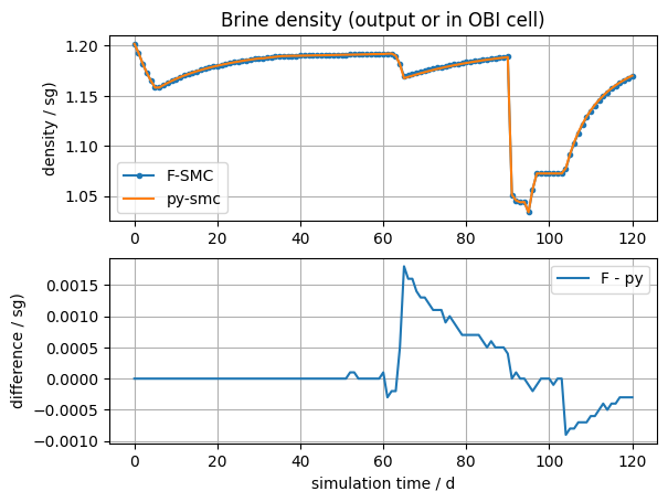
plt.subplot(2, 1, 1)
plt.title("Brine density (output or in OBI cell)")
plt.plot(tstF.t_d, tstF.sg_out, label="F-SMC", marker=".")
plt.plot(tstPy.t_d, tstPy.sg_out, label="py-smc")
plt.ylabel("density / sg)")
plt.grid()
_ = plt.legend()
plt.subplot(2, 1, 2)
plt.plot(tstF.t_d, tstF.sg_out - tstPy.sg_out, label="F - py")
plt.ylabel("difference / sg)")
plt.xlabel("simulation time / d")
plt.grid()
_ = plt.legend()
[6]:
plt.subplot(2, 1, 1)
plt.title("Average cavern brine density")
plt.plot(tstF.t_d, tstF.sg_ave, label="F-SMC", marker=".")
plt.plot(tstPy.t_d, tstPy.sg_ave, label="py-smc")
plt.ylabel("density / sg")
plt.grid()
_ = plt.legend()
plt.subplot(2, 1, 2)
plt.plot(tstF.t_d, tstF.sg_ave - tstPy.sg_ave, label="F - py")
plt.ylabel("difference / sg")
plt.xlabel("simulation time / d")
plt.grid()
_ = plt.legend()

[7]:
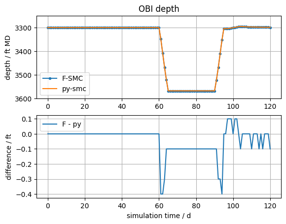
plt.subplot(2, 1, 1)
plt.title("OBI depth")
plt.plot(tstF.t_d, tstF.z_obi, label="F-SMC", marker=".")
plt.plot(tstPy.t_d, tstPy.z_obi, label="py-smc")
plt.ylabel("depth / ft MD")
plt.ylim(3600, 3250)
plt.grid()
_ = plt.legend()
plt.subplot(2, 1, 2)
plt.plot(tstF.t_d, tstF.z_obi - tstPy.z_obi, label="F - py")
plt.ylabel("difference / ft")
plt.xlabel("simulation time / d")
plt.grid()
_ = plt.legend()
[8]:
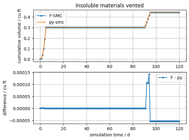
plt.subplot(2, 1, 1)
plt.title("Insoluble materials vented")
plt.plot(
    tstF.t_d,
    tstF.V_vented * sansmic.model.Units.cubic_foot() / sansmic.model.Units.barrel(),
    label="F-SMC",
    marker=".",
)
plt.plot(
    tstPy.t_d,
    tstPy.V_vented * sansmic.model.Units.cubic_foot() / sansmic.model.Units.barrel(),
    label="py-smc",
)
plt.ylabel("cumulative volume / cu ft")
plt.grid()
_ = plt.legend()
plt.subplot(2, 1, 2)
plt.plot(
    tstF.t_d,
    (tstF.V_vented - tstPy.V_vented)
    * sansmic.model.Units.cubic_foot()
    / sansmic.model.Units.barrel(),
    label="F - py",
    marker=".",
)
plt.ylabel("difference / cu ft")
plt.xlabel("simulation time / d")
plt.grid()
_ = plt.legend()
[9]:
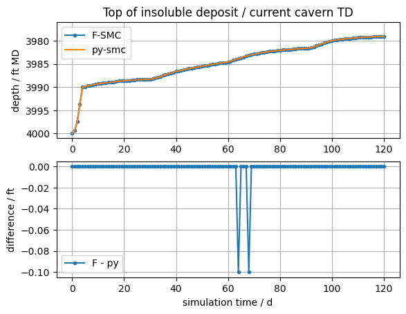
plt.subplot(2, 1, 1)
plt.title("Top of insoluble deposit / current cavern TD")
plt.plot(tstF.t_d, tstF.z_insol, label="F-SMC", marker=".")
plt.plot(tstPy.t_d, tstPy.z_insol, label="py-smc")
plt.ylabel("depth / ft MD")
plt.ylim(4001, 3976)
plt.grid()
_ = plt.legend()
plt.subplot(2, 1, 2)
plt.plot(tstF.t_d, tstF.z_insol - tstPy.z_insol, label="F - py", marker=".")
plt.ylabel("difference / ft")
plt.xlabel("simulation time / d")
plt.grid()
_ = plt.legend()
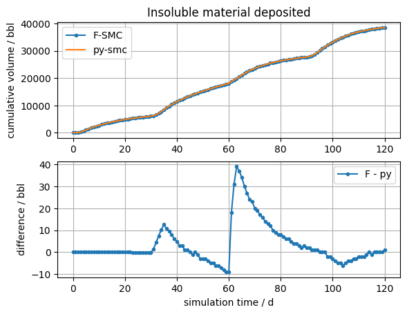
[10]:
plt.subplot(2, 1, 1)
plt.title("Insoluble material deposited")
plt.plot(tstF.t_d, tstF.V_insol, label="F-SMC", marker=".")
plt.plot(resPy.time, resPy.df_t_1D.V_insol, label="py-smc")
plt.ylabel("cumulative volume / bbl")
plt.grid()
_ = plt.legend()
plt.subplot(2, 1, 2)
plt.plot(tstF.t_d, tstF.V_insol - tstPy.V_insol, label="F - py", marker=".")
plt.ylabel("difference / bbl")
plt.xlabel("simulation time / d")
plt.grid()
_ = plt.legend()
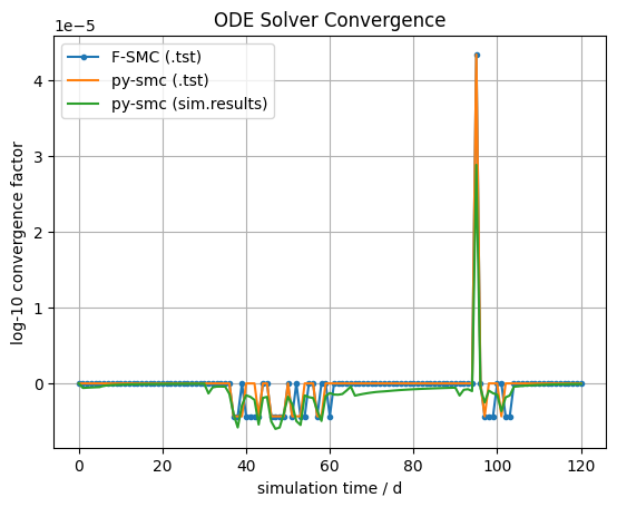
[11]:
plt.title("ODE Solver Convergence")
plt.plot(tstF.t_d, np.log10(tstF.err_ode), label="F-SMC (.tst)", marker=".")
plt.plot(tstPy.t_d, np.log10(tstPy.err_ode), label="py-smc (.tst)")
plt.plot(resPy.time, np.log10(resPy.df_t_1D.err_ode), label="py-smc (sim.results)")
plt.ylabel("log-10 convergence factor")
plt.xlabel("simulation time / d")
plt.grid()
_ = plt.legend()
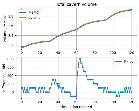
[12]:
plt.subplot(2, 1, 1)
plt.title("Total cavern volume")
plt.plot(tstF.t_d, tstF.V_cav / 1000000, label="F-SMC", marker=".")
plt.plot(tstPy.t_d, tstPy.V_cav / 1000000, label="py-smc")
plt.ylabel("volume / MMbbl")
plt.grid()
_ = plt.legend()
plt.subplot(2, 1, 2)
plt.plot(tstF.t_d, (tstF.V_cav - tstPy.V_cav), label="F - py", marker=".")
plt.ylabel("difference /   bbl")
plt.xlabel("simulation time / d")
plt.grid()
_ = plt.legend()
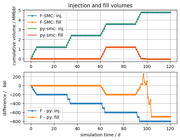
[13]:
plt.subplot(2, 1, 1)
plt.title("Injection and fill volumes")
plt.plot(tstF.t_d, tstF.V_inj / 1000000, label="F-SMC: inj.", marker=".")
plt.plot(tstF.t_d, tstF.V_fill / 1000000, label="F-SMC: fill", marker=".")
plt.plot(tstPy.t_d, tstPy.V_inj / 1000000, label="py-smc: inj.")
plt.plot(tstPy.t_d, tstPy.V_fill / 1000000, label="py-smc: fill")
plt.ylabel("cumulative volume / MMbbl")
plt.grid()
_ = plt.legend()
plt.subplot(2, 1, 2)
plt.plot(tstF.t_d, (tstF.V_inj - tstPy.V_inj), label="F - py: inj.", marker=".")
plt.plot(tstF.t_d, (tstF.V_fill - tstPy.V_fill), label="F - py: fill", marker=".")
plt.ylabel("difference /   bbl")
plt.xlabel("simulation time / d")
plt.grid()
_ = plt.legend()
[14]:
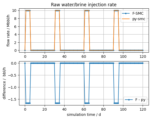
plt.subplot(2, 1, 1)
plt.title("Raw water/brine injection rate")
plt.plot(tstF.t_d, tstF.Q_inj / 24000, label="F-SMC", marker=".")
plt.plot(tstPy.t_d, tstPy.Q_inj / 24000, label="py-smc")
plt.ylabel("flow rate / Mbbl/h")
plt.grid()
_ = plt.legend()
plt.subplot(2, 1, 2)
plt.plot(tstF.t_d, (tstF.Q_inj - tstPy.Q_inj) / 24, label="F - py", marker=".")
plt.ylabel("difference / bbl/h")
plt.xlabel("simulation time / d")
plt.grid()
_ = plt.legend()
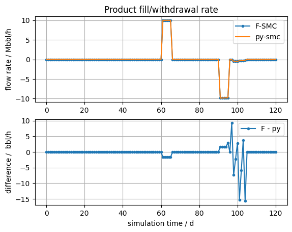
plt.figure()
plt.subplot(2, 1, 1)
plt.title("Product fill/withdrawal rate")
plt.plot(tstF.t_d, tstF.Q_fill / 24000, label="F-SMC", marker=".")
plt.plot(tstPy.t_d, tstPy.Q_fill / 24000, label="py-smc")
plt.ylabel("flow rate / Mbbl/h")
plt.grid()
_ = plt.legend()
plt.subplot(2, 1, 2)
plt.plot(tstF.t_d, (tstF.Q_fill - tstPy.Q_fill) / 24, label="F - py", marker=".")
plt.ylabel("difference / bbl/h")
plt.xlabel("simulation time / d")
plt.grid()
_ = plt.legend()
[15]:
Stats = sansmic.model.pd.DataFrame.from_dict(
    dict(
        rmse=np.sqrt(np.mean((tstF - tstPy) ** 2, 0)),
        min_F=tstF.min(),
        min_Py=tstPy.min(),
        max_F=tstF.max(),
        max_Py=tstPy.max(),
    )
)
Stats
[15]:
| rmse | min_F | min_Py | max_F | max_Py | |
|---|---|---|---|---|---|
| t_d | 0.000000 | 4.166700e-04 | 4.166700e-04 | 1.200000e+02 | 1.200000e+02 |
| V_cav | 219.126742 | 3.161000e+06 | 3.160900e+06 | 3.932200e+06 | 3.932200e+06 |
| err_ode | 0.000003 | 9.999900e-01 | 9.999900e-01 | 1.000100e+00 | 1.000100e+00 |
| sg_out | 0.000518 | 1.033800e+00 | 1.033900e+00 | 1.201900e+00 | 1.201900e+00 |
| sg_ave | 0.000133 | 1.125600e+00 | 1.125200e+00 | 1.201900e+00 | 1.201900e+00 |
| V_insol | 9.851207 | 1.153100e-05 | 1.153100e-05 | 3.856000e+04 | 3.855900e+04 |
| z_insol | 0.012856 | 3.979100e+03 | 3.979100e+03 | 4.000000e+03 | 4.000000e+03 |
| z_obi | 0.096638 | 3.295100e+03 | 3.295200e+03 | 3.567500e+03 | 3.567600e+03 |
| V_vented | 0.000175 | 7.906800e-08 | 7.906800e-08 | 2.497900e+00 | 2.498200e+00 |
| Q_inj | 16.262313 | 0.000000e+00 | 0.000000e+00 | 2.399600e+05 | 2.400000e+05 |
| Q_fill | 58.221127 | -2.373700e+05 | -2.374100e+05 | 2.399600e+05 | 2.400000e+05 |
| V_inj | 534.959642 | 9.998300e+01 | 1.000000e+02 | 4.799200e+06 | 4.800000e+06 |
| V_fill | 284.917040 | -4.601500e+04 | -4.531800e+04 | 1.199800e+06 | 1.200000e+06 |
[16]:
logStats = np.log10(abs(Stats))
finalDigit = (np.power(10, logStats["rmse"] - logStats["max_F"]) * 1000000 // 10) / 10
finalDigit.name = "average difference in last of 5 digits"
finalDigit.astype(int)
/opt/hostedtoolcache/Python/3.12.10/x64/lib/python3.12/site-packages/pandas/core/internals/blocks.py:393: RuntimeWarning: divide by zero encountered in log10
  result = func(self.values, **kwargs)
[16]:
t_d         0
V_cav       0
err_ode     0
sg_out      4
sg_ave      1
V_insol     2
z_insol     0
z_obi       0
V_vented    0
Q_inj       0
Q_fill      2
V_inj       1
V_fill      2
Name: average difference in last of 5 digits, dtype: int64
The average difference in the last digit printed is shown above as D in X.XXXDe±XX. Values less than 2.0 indicate the average difference is less than the FORTAN-SANSMIC program’s output accuracy.
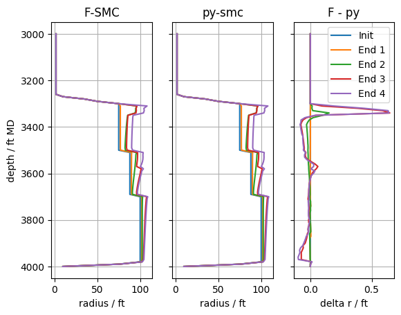
Full output differences#
[17]:
plt.subplot(1, 3, 1)
plt.title("F-SMC")
plt.plot(resF.radius[0], resF.depths, label="1 d")
plt.plot(resF.radius[29], resF.depths, label="30 d")
plt.plot(resF.radius[59], resF.depths, label="60 d")
plt.plot(resF.radius[89], resF.depths, label="90 d")
plt.plot(resF.radius[119], resF.depths, label="120 d")
plt.ylim(4050, 2950)
plt.ylabel("depth / ft MD")
plt.xlabel("radius / ft")
plt.grid()
plt.subplot(1, 3, 2)
plt.title("py-smc")
plt.plot(resPy.radius[1], resPy.depths, label="1 d")
plt.plot(resPy.radius[30], resPy.depths, label="30 d")
plt.plot(resPy.radius[60], resPy.depths, label="60 d")
plt.plot(resPy.radius[90], resPy.depths, label="90 d")
plt.plot(resPy.radius[120], resPy.depths, label="120 d")
plt.ylim(4050, 2950)
plt.xlabel("radius / ft")
plt.grid()
plt.yticks([4000, 3800, 3600, 3400, 3200, 3000], ["", "", "", "", "", ""])
plt.subplot(1, 3, 3)
plt.title("F - py")
plt.plot(resF.radius[0] - resPy.radius[1], resF.depths, label="Init")
plt.plot(resF.radius[29] - resPy.radius[30], resF.depths, label="End 1")
plt.plot(resF.radius[59] - resPy.radius[60], resF.depths, label="End 2")
plt.plot(resF.radius[89] - resPy.radius[90], resF.depths, label="End 3")
plt.plot(resF.radius[119] - resPy.radius[120], resF.depths, label="End 4")
plt.legend()
plt.ylim(4050, 2950)
plt.yticks([4000, 3800, 3600, 3400, 3200, 3000], ["", "", "", "", "", ""])
plt.grid()
_ = plt.xlabel("delta r / ft")
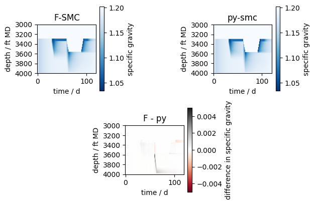
[18]:
plt.subplot(2, 3, 1)
plt.imshow(resF.cell_sg)
plt.title("F-SMC")
plt.ylim(0, 100)
plt.ylabel("depth / ft MD")
plt.xlabel("time / d")
plt.yticks([0, 20, 40, 60, 80, 100], labels=["4000", "3800", "3600", "3400", "3200", "3000"])
plt.colorbar(label="specific gravity")
plt.set_cmap("Blues_r")
plt.subplot(2, 3, 3)
plt.imshow(resPy.cell_sg)
plt.title("py-smc")
plt.ylim(0, 100)
plt.ylabel("depth / ft MD")
plt.xlabel("time / d")
plt.yticks([0, 20, 40, 60, 80, 100], labels=["4000", "3800", "3600", "3400", "3200", "3000"])
plt.colorbar(label="specific gravity")
plt.set_cmap("Blues_r")
plt.subplot(2, 3, 5)
plt.imshow(
    resF.cell_sg.iloc[:, :].T.reset_index(drop=True).T
    - resPy.cell_sg.iloc[:, 1:].T.reset_index(drop=True).T
)
plt.title("F - py")
plt.ylim(0, 100)
plt.ylabel("depth / ft MD")
plt.xlabel("time / d")
plt.yticks([0, 20, 40, 60, 80, 100], labels=["4000", "3800", "3600", "3400", "3200", "3000"])
plt.colorbar(label="difference in specific gravity")
plt.clim(-0.005, 0.005)
plt.set_cmap("RdGy")
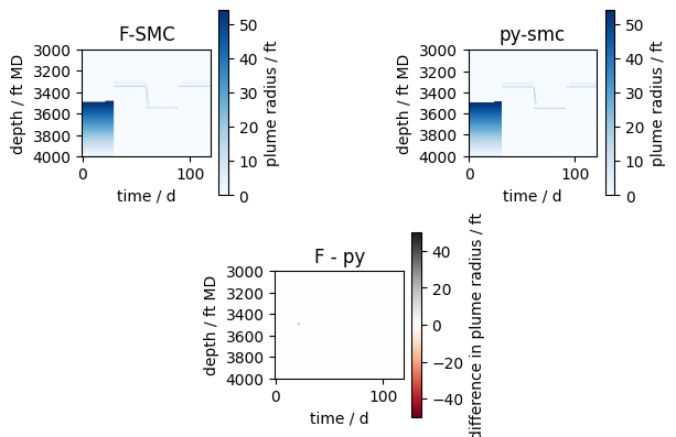
[19]:
plt.subplot(2, 3, 1)
plt.imshow(resF.plume_radius)
plt.title("F-SMC")
plt.ylim(0, 100)
plt.ylabel("depth / ft MD")
plt.xlabel("time / d")
plt.yticks([0, 20, 40, 60, 80, 100], labels=["4000", "3800", "3600", "3400", "3200", "3000"])
plt.colorbar(label="plume radius / ft")
plt.set_cmap("Blues")
plt.subplot(2, 3, 3)
plt.imshow(resPy.plume_radius)
plt.title("py-smc")
plt.ylim(0, 100)
plt.ylabel("depth / ft MD")
plt.xlabel("time / d")
plt.yticks([0, 20, 40, 60, 80, 100], labels=["4000", "3800", "3600", "3400", "3200", "3000"])
plt.colorbar(label="plume radius / ft")
plt.set_cmap("Blues")
plt.subplot(2, 3, 5)
plt.imshow(
    resF.plume_radius.iloc[:, :].T.reset_index(drop=True).T
    - resPy.plume_radius.iloc[:, 1:].T.reset_index(drop=True).T
)
plt.title("F - py")
plt.ylim(0, 100)
plt.ylabel("depth / ft MD")
plt.xlabel("time / d")
plt.yticks([0, 20, 40, 60, 80, 100], labels=["4000", "3800", "3600", "3400", "3200", "3000"])
plt.colorbar(label="difference in plume radius / ft")
plt.clim(-50, 50)
plt.set_cmap("RdGy")
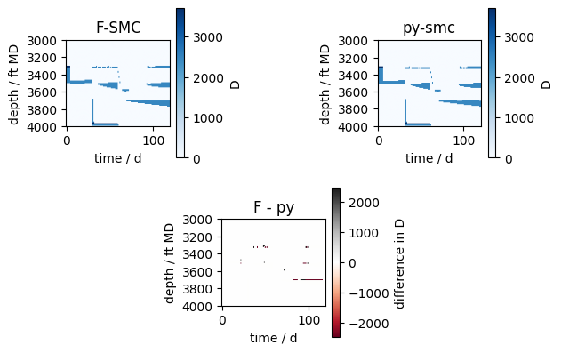
[20]:
plt.subplot(2, 3, 1)
plt.imshow(resF.effective_diffusion_coefficient)
plt.title("F-SMC")
plt.ylim(0, 100)
plt.ylabel("depth / ft MD")
plt.xlabel("time / d")
plt.yticks([0, 20, 40, 60, 80, 100], labels=["4000", "3800", "3600", "3400", "3200", "3000"])
plt.colorbar(label="D")
plt.set_cmap("Blues")
plt.subplot(2, 3, 3)
plt.imshow(resPy.effective_diffusion_coefficient)
plt.title("py-smc")
plt.ylim(0, 100)
plt.ylabel("depth / ft MD")
plt.xlabel("time / d")
plt.yticks([0, 20, 40, 60, 80, 100], labels=["4000", "3800", "3600", "3400", "3200", "3000"])
plt.colorbar(label="D")
plt.set_cmap("Blues")
plt.subplot(2, 3, 5)
plt.imshow(
    resF.effective_diffusion_coefficient.iloc[:, :].T.reset_index(drop=True).T
    - resPy.effective_diffusion_coefficient.iloc[:, 1:].T.reset_index(drop=True).T
)
plt.title("F - py")
plt.ylim(0, 100)
plt.ylabel("depth / ft MD")
plt.xlabel("time / d")
plt.yticks([0, 20, 40, 60, 80, 100], labels=["4000", "3800", "3600", "3400", "3200", "3000"])
plt.colorbar(label="difference in D")
plt.set_cmap("RdGy")
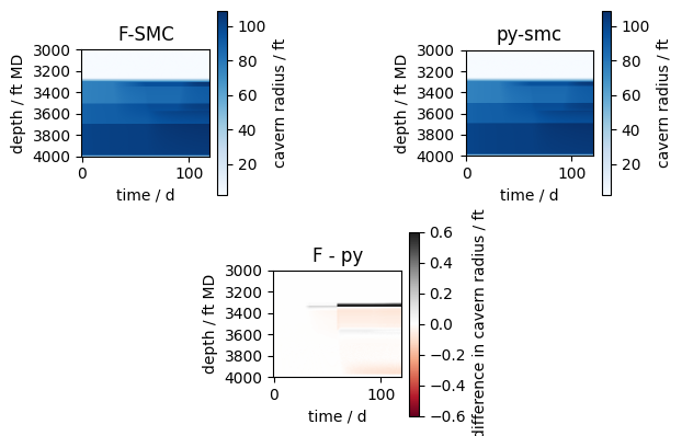
[21]:
plt.subplot(2, 3, 1)
plt.imshow(resF.radius)
plt.title("F-SMC")
plt.ylim(0, 100)
plt.ylabel("depth / ft MD")
plt.xlabel("time / d")
plt.yticks([0, 20, 40, 60, 80, 100], labels=["4000", "3800", "3600", "3400", "3200", "3000"])
plt.colorbar(label="cavern radius / ft")
plt.set_cmap("Blues")
plt.subplot(2, 3, 3)
plt.imshow(resPy.radius)
plt.title("py-smc")
plt.ylim(0, 100)
plt.ylabel("depth / ft MD")
plt.xlabel("time / d")
plt.yticks([0, 20, 40, 60, 80, 100], labels=["4000", "3800", "3600", "3400", "3200", "3000"])
plt.colorbar(label="cavern radius / ft")
plt.set_cmap("Blues")
plt.subplot(2, 3, 5)
plt.imshow(
    resF.radius.iloc[:, :].T.reset_index(drop=True).T
    - resPy.radius.iloc[:, 1:].T.reset_index(drop=True).T
)
plt.title("F - py")
plt.ylim(0, 100)
plt.ylabel("depth / ft MD")
plt.xlabel("time / d")
plt.yticks([0, 20, 40, 60, 80, 100], labels=["4000", "3800", "3600", "3400", "3200", "3000"])
plt.colorbar(label="difference in cavern radius / ft")
plt.clim(-0.6, 0.6)
plt.set_cmap("RdGy")
[ ]: