3Using Rattlesnake
This chapter will describe how to use Rattlesnake through its user interface (UI). Rattlesnake is capable of running several different types of control, therefore the UI may look different for different tests. In general, the UI consists of a tabbed interface across the top of the main window, and users must complete each tab before proceeding to the next. The tabs that exist in a given test will depend on which control type is being run. For example, in a combined environments test (see Chapter 19) such as the one shown in Figure 3.1), there is a Test Profile tab that allows the user to define a testing timeline. Additionally, environments such as the MIMO Random Vibration environment (see Chapter 12) require a system identification phase where the controller identifies relationships between the output signals and the control degrees of freedom. Therefore, tests using the MIMO Random Vibration environment will also have a System Identification and Test Predictions tab. Figure 3.2, on the other hand, shows the UI for a test that only utilizes the Time History environment (see Chapter 17) so these optional tabs are not displayed.

Figure 3.1:Rattlesnake UI tabs when running a combined environments test with an environment that requires a system identification.

Figure 3.2:Rattlesnake UI tabs when running a single environment with no system identification phase.
Users of Rattlesnake must be aware that depending on their test configuration, their UI may not appear identical to images shown in this User’s Manual. Additionally, users should be aware that the UI library used by this software will inherit stylistic features from the operating system. There may therefore be cosmetic differences between the images of the UI shown in this document and the UI seen by the user. All images in this document were created using Microsoft Windows 10 or Windows 11 operating systems, so users with Mac or Linux operating systems will note a difference in UI appearance.
Note that the Rattlesnake enforces an order to operations when defining a particular test by enabling and disabling tabs in the UI. Initially, only the first tab will be enabled. As the users complete each tab, the next tab will become available. In Figure 3.1 and Figure 3.2, it can be seen that only the initial tabs are enabled, and subsequent tabs are disabled.
Once all tabs are enabled, Rattlesnake continues to employ a state tracking paradigm which will not allow users to perform an invalid operation. For example if users are actively running a test and return to the Environment Definition tab, trying to re-initialize environments will result in a state error.
3.1Global Data Acquisition Settings
The Data Acquisition Setup tab of the Rattlesnake UI specifies the global test parameters that the controller will use. Parameters are determined to be global when they affect all environments or the controller itself. The three main sections of this portion of the interface are the Channel Table, Environment Table, and Global Data Acquisition Parameters. Figure 3.3 shows this.
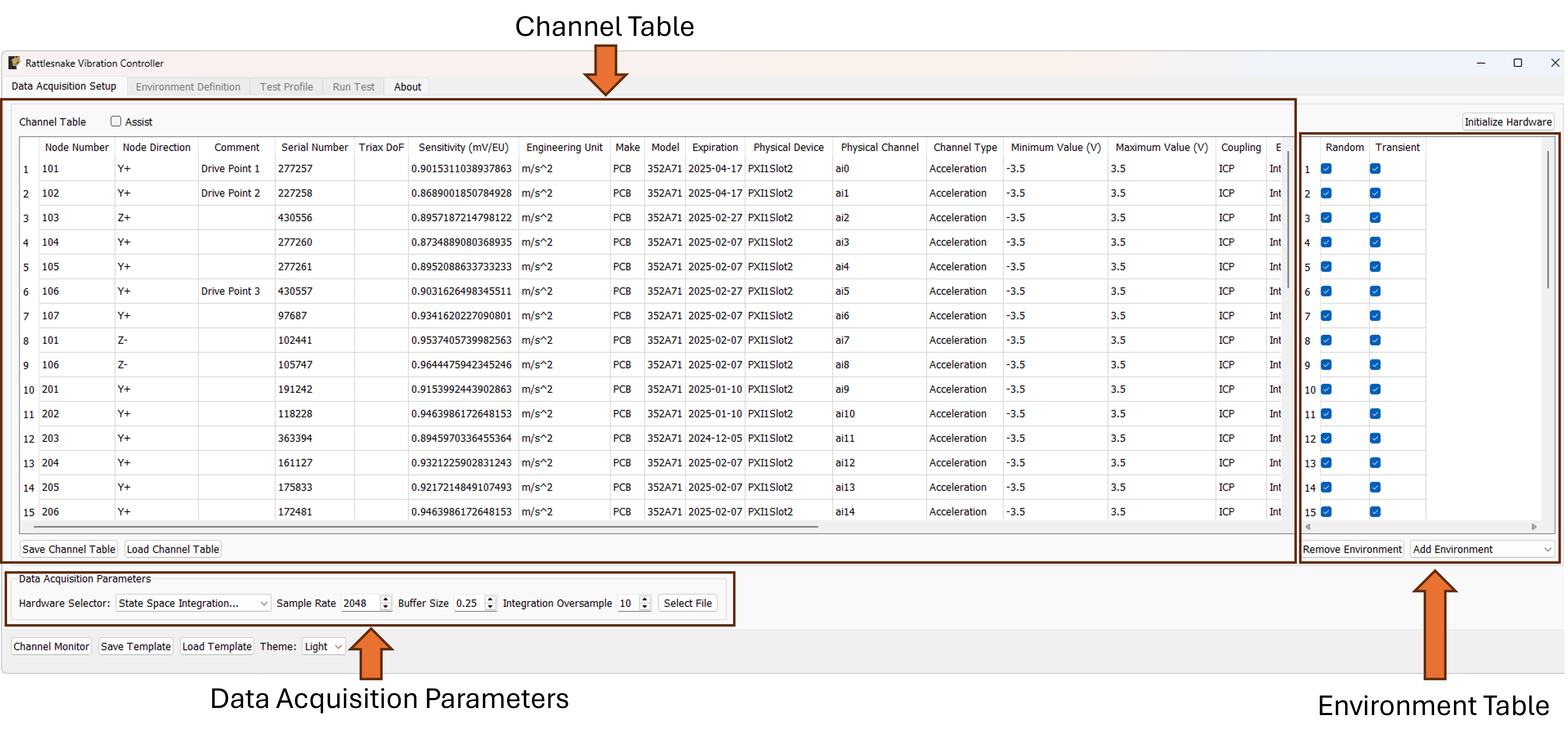
Figure 3.3:Data Acqisition Setup tab in the Rattlesnake Controller where the Channel Table, Environment Table, and Data Acquisition Parameters are specified.
3.1.1Channel Table
The channel table specifies how the instrument channels in a given test are connected to the data acquisition hardware, as well as how the data read from those channels are used by the software.
In general, for a given test there will be a set of excitation devices that use the output signals from Rattlesnake as well as instrumentation to record the test article’s responses to those exciters. Rattlesnake requires each instrument (or each channel on each instrument for multi-axial instruments) as well as each excitation device to have a row in the channel table. This is perhaps contrary to other control software where only the response channels need to be set up in the channel table. However, to maintain the flexibility to run multiple types of hardware devices, some of which having limitations to their triggering capabilities, Rattlesnake must read in the signal from its output directly in order to be able to synchronize its outputs and the responses to those outputs. Therefore, for all Rattlesnake test setups, the output signal should be split using a tee to the exciter and the corresponding input channel. Because of this requirement, one should keep in mind that the number of acquisition channels required on the hardware device for a given test is actually the number of responses plus the number of outputs. Figure 3.4 shows a schematic of a four acquisition channel, two output channel LAN-XI module set up for use with Rattlesnake.
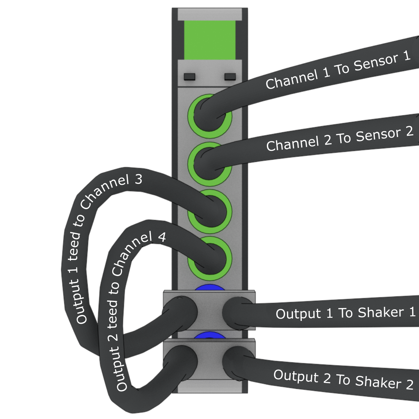
Figure 3.4:Output channels teed to acquisition channels so they can be read by the controller.
The required data input into the channel table varies with the physical or virtual hardware used for the test. For device-specific channel table requirements, see the appropriate section of Part 2: Rattlesnake Hardware Devices. In general, the entries to the channel table are as follows:
Node Number Determines the instrumentation position on the test article. The node number will generally correspond to a node in a test geometry or FEM. While not used directly by the controller for most environments except to label plots, it is important for book-keeping and test documentation. The modal environment does use this value when identifying drive point measurements.
Node Direction Determines the instrumentation direction on the test article at the position specified by the Node Number. The Node Direction will generally correspond to the node’s local coordinate system if one exists in the test geometry. While not used directly by the controller for most environments except to label plots, it is important for book-keeping and test documentation. The modal environment does use this value when identifying drive point measurements.
Comment Provides space for additional information about a channel that may not be captured by the Node Number and Node Direction.
Serial Number The serial number of the instrument used for the given channel. This field is not used by the controller but will be stored with the test data and is important for data traceability to know which instruments were used to measure which channels.
Triax DoF The degree of freedom on a given instrument corresponding to the given channel. This is primarily used to distinguish between the three axes of a triaxial accelerometer, but has the potential to be used for other multi-axis instrumentation types such as strain gauge rosettes.
Sensitivity The sensitivity of the instrument in millivolts per Engineering Unit. This is used to transform the acquired data from a raw voltage to a engineering quantity such as acceleration or force.
Engineering Unit The unit in which the measured signal for the given instrument will be reported. Certain hardware will limit the units that can be specified: see Part 2: Rattlesnake Hardware Devices for more information.
Make The name of the instrument’s manufacturer, used for data traceability.
Model The product name or model number of the instrument, used for data traceability.
Expiration The expiration date of the instrument’s calibration certificate. Note that this is only for data traceability; no checking of this date with the current data to ensure a valid calibration is performed by the software.
Physical Device The reference to a physical device attached to the computer. The entries in this field will be specific to the acquisition hardware being used for a given test. For virtual control, this column must be filled to specify that a given channel is active. See Part 2: Rattlesnake Hardware Devices for more information.
Physical Channel The reference to a channel on a physical device attached to the computer. The entries in this column will be specific to the acquisition hardware being used for a given test. See Part 2: Rattlesnake Hardware Devices for more information.
Channel Type The type of the channel being used for a given test, such as Acceleration, Force, or Voltage. The allowable entries in this column will be specific to the acquisition hardware being used for a given test. See Part 2: Rattlesnake Hardware Devices for more information.
Minimum Value (V) The minimum voltage that the data acquisition system can handle during a test. This is used to set the range on the data acquisition system. For hardware devices with symmetric ranges (e.g. ±10V), this column can be left blank.
Maximum Value (V)] The maximum voltage that the data acquisition system can handle during a test. This is used to set the range on the data acquisition system. For hardware devices with symmetric ranges (e.g. ±10V), this column is used to set the maximum and minimum voltage values.
Coupling The coupling used by the data acquisition system. This may include filtering in addition to AC/DC coupling, which is dependent on the hardware being used for a given test. See Part 2: Rattlesnake Hardware Devices for more information.
Excitation Source Used to specify the signal conditioning that is required by the instrument. This column is generally where the constant current line drive (CCLD)/integrated electronics piezoelectric (IEPE)/integrated circuit piezoelectric (ICP) is specified for a given hardware device. See Part 2: Rattlesnake Hardware Devices for more information.
Current Excitation (A) Used to specify the excitation current sent to the device for signal conditioning. Depending on whether the device has a fixed or variable excitation current, this field may be left empty. This can also be left empty if no signal conditioning is provided by the data acquisition system. See Part 2: Rattlesnake Hardware Devices for more information.
Feedback Device For output channels, this is the reference to the output or excitation device that is being fed back into the current channel’s Physical device. If the current channel is not an output channel, it should be left empty. A populated Feedback Device column tells the controller that the given channel is an output channel.
Feedback Channel For output channels, this is the reference to the output channel on the output or excitation device that is being fed back into the current channel’s Physical Device. As an example using generic device and channel names, if
Channel 2onGenerator 1is teed off toChannel 3onAcquisition Card 2, the corresponding row in the channel table would haveAcquisition Card 2specified as the Physical Device,Channel 3specified as the Physical Channel,Generator 1specified as theFeedback DeviceandChannel 2specified as the feedback channel.Warning Level A warning level can be implemented for each channel. The warning level is specified in the same units as the Engineering Unit column. When a channel hits the warning limit, it will be flagged as Yellow in the Channel Monitor (see Section 3.9). The warning level can be left blank if no warning is desired.
Abort Level An abort level can be implemented for each channel. The abort level is specified in the same units as the Engineering Unit column. When a channel hits the abort limit, it will be flagged as Red in the Channel Monitor (see Section 3.9). The controller will also shut down if an abort level is reached. The abort level can be left blank if no abort is desired.
To limit the tediousness of inputting channel table information into the UI by hand, the channel table can be loaded from an Excel spreadsheet or Comma-separated-value file. A channel table can be loaded by clicking the Load Channel Table button under the channel table, which will bring up a file selection dialog, enabling the user to select a file to load. For convenience, a template Excel spreadsheet is attached to this page:
A template Excel file can also be generated by creating a test in Rattlesnake and saving the empty channel table by clicking the Save Channel Table button under the channel table. If a channel table is filled out in Rattlesnake’s UI, its contents will be saved to the file as well.
3.1.2Environment Table
In order to run a test, it must be populated with one or more environments. An environment is effectively the type of control that the controller provides. For example, the MIMO Random environment controls the test article to a specified CPSD matrix, while the MIMO Transient controls the test article to a specified time history.
Environments can be added to the test by clicking the Add Environment dropdown and selecting the type of environment that is desired, as shown in Figure 3.5.
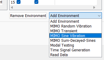
Figure 3.5:Adding an environment to the Rattlesnake controller.
When an environment type is selected, a dialog box will appear querying the user for the name of the environment, as shown in Figure 3.6.
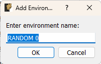
Figure 3.6:Defining the name of the new environment.
As environments are added, their names will appear as the columns of the Environment Table. Rows of this table will be populated with checkboxes; a checked checkbox will indicate that the channel corresponding to the checkbox’s row is used for the environment corresponding to the checkbox’s column. A channel can be used for multiple environments, a single environment, or no environments. Channels used by no environments will still be measured and streamed to disk, but will not be sent to any environment for use in the respective control approaches. The environment table is also used to specify which excitation devices are used by which environment.
For single environment tests, the software assumes that all channels in the channel table are used by the single environment regardless of checkbox state.
3.1.3Data Acquisition Parameters
The final portion of Data Acquisition Setup tab specifies data acquisition parameters. These parameters may change depending on the hardware selected.
Hardware Selector The physical or virtual hardware used for the test. See Part 2: Rattlesnake Hardware Devices for hardware specific details of the controller. For some devices, a file selector window will appear will appear when the device is selected, as that device needs more information to operate. This is primarily the case for virtual hardware where some model of the test article must be loaded. This is also used when a specific hardware device needs to access external functionality in a library such as a
dllfile or requires a license file.Sample Rate The sample rate of the hardware devices used for the test. Some devices will have arbitrary sample rates, and some devices have fixed sample rates, so the options available will depend on the acquisition hardware being used.
Buffer Size The amount of data that the acquisition system will acquire or output with each read from or write to the hardware. By reading and writing data in chunks, hardware input/output operations with relatively large overhead can be limited, and the buffer gives the controller time to catch up if e.g. the operating system decides to start a computationally intensive task in the background of the computer. Note that specifying large numbers for this quantity (e.g. 10 seconds) will reduce the responsiveness of the controller, because the controller will potentially not receive the acquired data until 10 seconds after it was acquired. Note also that this value does not need to correspond to the Samples per Analysis Frame or any other signal processing parameter used by an environment. Each environment should be buffered such that it creates appropriately sized analysis windows from the differently sized acquisition chunks.
Hardware Specific Parameters Depending on the hardware device selected, additional UI elements may appear in the
Data Acquisition Parameterssection of the window. See the Chapter in Part 2: Rattlesnake Hardware Devices corresponding to the hardware device in use for information on these hardware-specific parameters.
3.1.4Initialize Hardware
With the Data Acquisition Settings specified in the UI, the Data Acquisition can be initialized by pressing the Initialize Hardware button in the top-right corner of the window. At this point, the controller will go through and create the programming interfaces to the hardware device, specify the sampling parameters, and create the channels on the devices. It will also update the UI given the environments specified in the test. The software will then proceed to the next tab.
Figure 3.7 and Figure 3.8 show a completed Data Acquisition Setup tab with twenty accelerometer response channels, three force response channels, and three voltage drive channels that have been teed into acquisition channels. It also contains two environments, Random and Shock, which both have all response channels and all drive channels active for them.
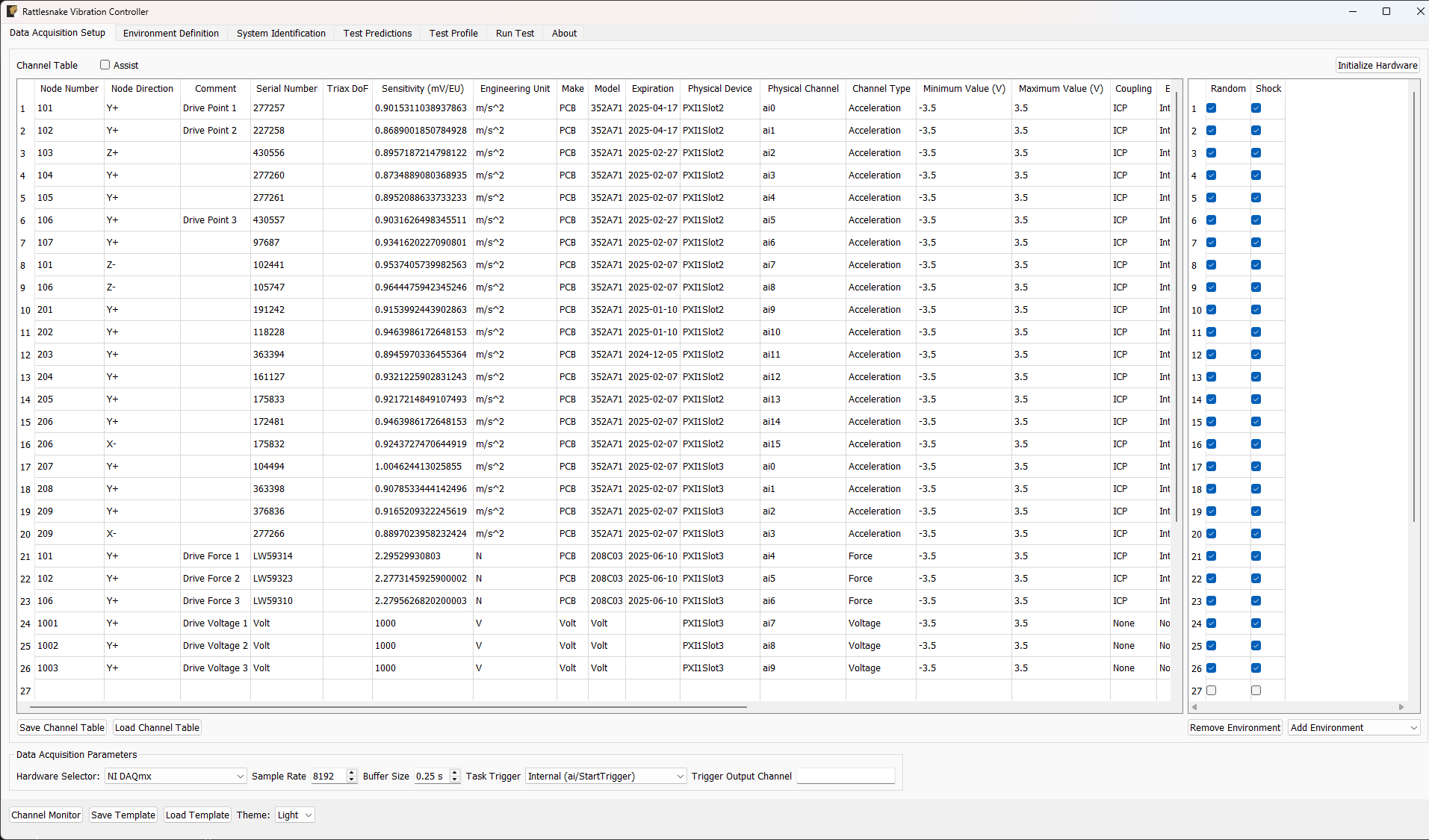
Figure 3.7:Example of a completed Data Acquisition Setup tab with three response channels and one output channel.
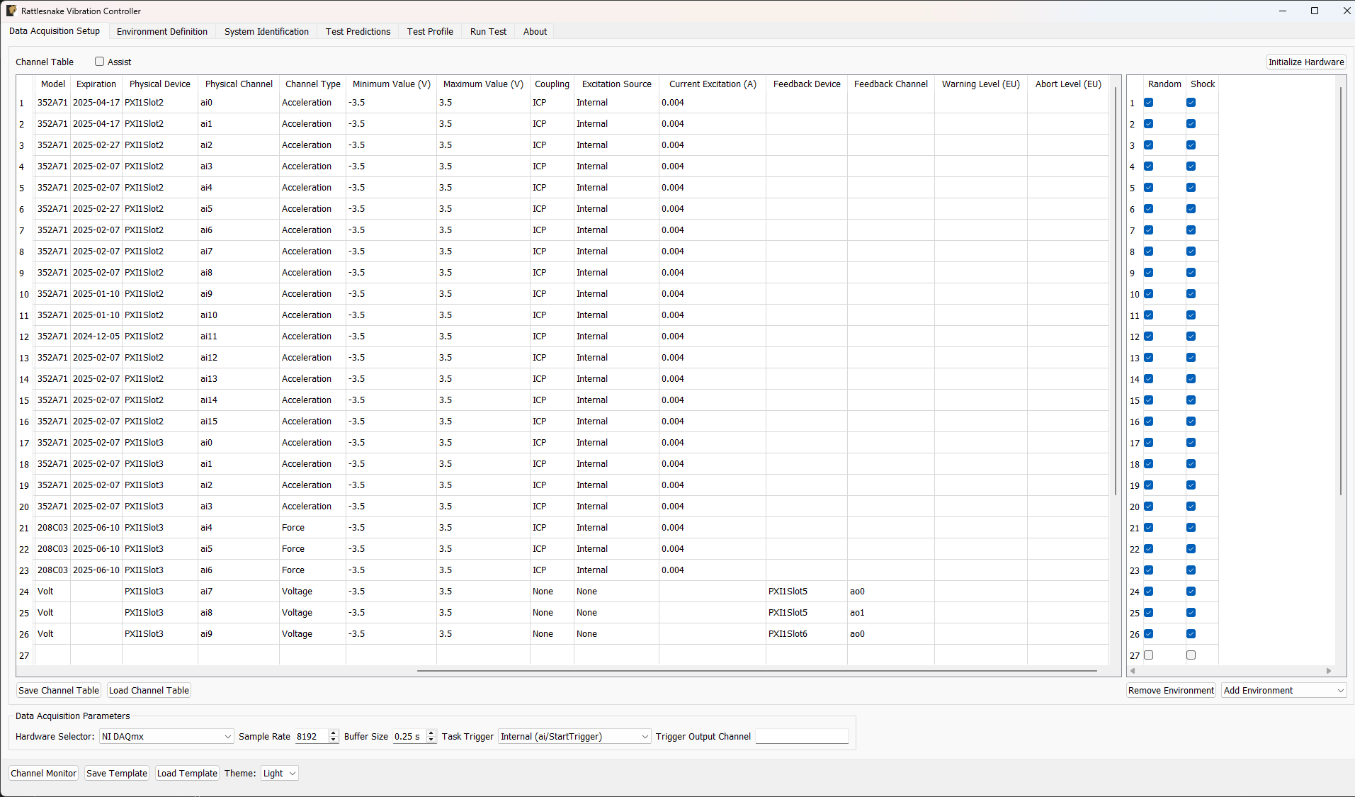
Figure 3.8:Continuation of Figure 3.7 with the channel table scrolled to see additional columns.
3.2Environment Definition
The Environment Definition tab is the second tab in the Rattlesnake software. It is in this tab that the various environments are defined. The main tab will have one sub-tab for each environment, as shown in Figure 3.9.
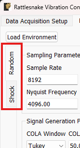
Figure 3.9:Sub-tabs for environments Random and Shock in the Environment Definition tab.
Different environment types will have different parameters that can be set. See Part 3: Rattlesnake Environments for a description of each environment type in Rattlesnake and the parameters that define it.
When all environments are defined, the Initialize Environments button in the top-right corner of the tab can be pressed to proceed to the next portion of the controller.
3.3System Identification
With the environments defined, the controller proceeds to the System Identification tab if required by any environment, shown in Figure 3.10. During this phase of the controller, the controller will develop relationships between the excitation signals and the responses of the test article to those excitation signals. It will also make a measurement of the noise floor of the test.
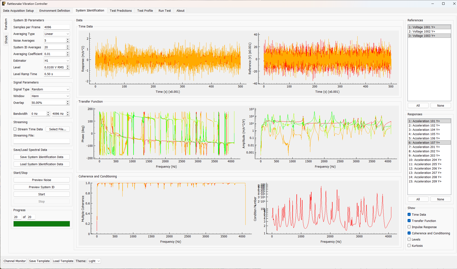
Figure 3.10:System identification tab showing various signals and spectral quantities that can be used to control and evaluate the test.
Not all environment types will require a system identification. For environments that simply stream excitation data, a system identification will generally not be required. However for any environment that aims to produce an excitation signal that creates some desired response on the test article, a system identification will be required to understand the relationships between the excitation signals and the response signals.
There will be one sub-tab for each environment that requires a System Identification. System identification must be run for each sub-tab before the test can be run. If no environment requires system identification, then the entire System Identification tab will be removed. When system identification is performed, the software will first perform a noise floor measurement, where all channels are recorded, but no excitation signal is provided. After the noise floor calculation completes, the system identification will begin.
There are many options that define how the system identification phase is performed.
3.3.1System Identification Parameters
The System ID Parameters section of the System Identification tab consists of the following parameters:
Samples per Frame Samples per measurement frame used in the system identification. Some environments force system identification to use the same frame size as the signal processing performed in the environment. If this field cannot be edited here, then check the Environment Definition tab for a similar property.
Averaging Type Type of averaging used in the system identification. Linear averaging weights each measurement frame equally. Exponential averaging treats more recent averages with a higher weight.
Noise Averages Number of measurement frames to acquire to analyze the noise level of the test.
System ID Averages Number of measurement frames to acquire to identify the system and compute transfer functions.
Averaging Coefficient Averaging coefficient used to weight the most recent measurement frame if exponential averaging is used.
Estimator The estimator to use to compute transfer functions when performing system identification.
Level Root-mean-square voltage level to play to the shakers when computing system identification
Ramp Time Time to ramp the system identification voltage to the test level.
3.3.2Signal Parameters
The System Identification tab also gives the option to select the signal to use for system identification. These options are shown in the Signal Parameters section of the tab. Some options are only shown if certain signal types are selected. For example, only a burst random excitation signal uses a trigger, so it is the only one where a pretrigger can be specified.
On Fraction Fraction of the measurement frame that the burst random excitation is active for.
Pretrigger Percentage of the measurement frame that is before the burst random excitation.
Ramp Fraction Percentage of the burst that is used to ramp from zero to the test level.
Signal Type Excitation used for system identification. Random and Burst random excitation are suitable for MIMO control problems. Chirp and Pseudorandom should only be used for single-shaker excitation.
Window Window function to apply to the data when computing transfer functions during system identification.
Overlap Overlap to use between measurement frames when computing transfer functions.
Bandwidth Minimum Frequency The lowest frequency content in the excitation signal used in system identification.
Bandwidth Maximum Frequency The highest frequency content in the excitation signal used in system identification.
3.3.3Streaming and Saving Spectral Data
Often it is of interest to save data from the system identification phase, either for offline processing or simply to document what was done to the test article. The system identification phase can stream time data to disk by selecting a streaming file and clicking the Stream Time Data checkbox. Data will be streamed to a netCDF4 file. If streaming time data, the noise measurement will be saved to the variable name time_data and the system identification measurement will be saved to the variable name time_data_1 (see Section 3.7 for more information on the structure of this file). Options for streaming data are found in the Streaming section of the tab.
Select File... Opens a file dialog to select the file to which the system identification data will be streamed.
Stream Time Data If checked, time data from system identification will be streamed to disk.
Streaming File: File to which system identification data will be streamed.
In addition to streaming time data, the spectral data from the system identification can be saved to disk by clicking the Save System Identification Data button and selecting the file. Users can also load system identification data, which is useful if system identification is a long-running phase of the control system, or the user does not want to put additional stress onto the test article. When loading system identification data, one must be careful that the loaded data has the same control and excitation degrees of freedom as the current environment, and that they are in the same order. Otherwise, the channels in the loaded data will not map correctly to the current environment. Operations to save and load system identification spectral data are found in the Save/Load Spectral Data portion of the tab.
Save System Identification Data Save system identification spectral data to a file on the disk.
Load System Identification Data Loads system identification data from a file on the disk. System identification being loaded must contain the same control and excitation degrees of freedom in the same order as the current environment.
3.3.4Running system identification
To run the system identification, there are buttons to Preview the Noise or System ID characterizations. When ready, the Start button can be clicked. It will run a Noise Characterization for the specified number of Noise Averages, and then subsequently run the System Identification characterization for the specified number of System ID Averages. Both of these operations will stop automatically when the specified number of averages is reached or may be aborted early by pressing the Stop button. If the user wishes to run either the noise or system identification phases continuously, they can click the Preview Noise or Preview System ID buttons. These previews will run continuously until the Stop button is pressed. These operations are found in the Start/Stop portion of the tab.
Preview Noise Starts the noise identification of the system identification process in preview mode. No excitation will be applied to the shakers. The preview will continue until stopped manually.
Preview System Identification Starts the system identification process in preview mode with excitation applied to the shakers. The preview will continue until stopped manually.
Start Starts the full system identification process, including noise characterization and transfer function computation. Each step will stop automatically when the requested number of averages has been acquired.
Stop Manually stops the system identification process.
As the system identification proceeds, the displays in the Progress portion of the tab will be updated.
Current Averages Current number of system identification averages that have been acquired.
Total Averages Total number of system identification averages that will be acquired.
System Identification Progress Bar Graphically displays the system identification’s progress for the current noise or system identification step.
Data will be plotted as the system identification proceeds. The channels to visualize can be selected by clicking one or more of the channels Responses or References on the right side of the screen.
In the Responses:
Responses Select the response channels to visualize on the plots on the System Identification tab.
All Visualize all responses.
None Visualize no responses.
In the References:
References Select the reference channels to visualize on the plots on the System Identification tab.
All Visualize all references.
None Visualize no references.
By default, Time Data and Transfer Functions are shown. However, additional quantities of interest can be shown by clicking on the checkboxes in the Show portion of the tab.
Time Data Check to show time data during the system identification.
Transfer Function Check to show transfer functions in the system identification.
Impulse Response Check to show the impulse response function, which is the IFFT of the transfer function.
Coherence and Conditioning Check to show multiple coherence and condition number of the transfer function matrix.
Levels Check to show levels for system identification and noise characterization
Kurtosis Check to show kurtosis of response and reference channels.
The plots that can be shown are:
Time Data Plot Displays the most recently acquired measurement frames for the selected reference and response channels.
Transfer Function Plot Displays the current estimation of the system transfer functions for the currently selected reference and response channels.
Impulse Response Plot Displays the current estimation of the impulse response function for the currently selected reference and response channels.
Coherence and Condition Number Plots Displays the multiple coherence for the currently selected response channel, and the condition number for each frequency line in the transfer function matrix.
Levels Plots Displays the levels of the selected response and reference channels compared to the noise level on that measurement.
Kurtosis Plot Displays the kurtosis of all channels in the system identification. A kurtosis of 3 suggests gaussian measurements. A value far from 3 suggests some nonlinear effect is distorting the gaussian excitation signals.
3.4Test Predictions
Once the system identification for each environment completes, the controller will compute a prediction for that environment. This prediction will be based on the measured transfer functions between output signals and measured responses, as well as the environment parameters specified on the Environment Definition tab. Predictions will typically be made both for excitation signals required as well as response accuracy, allowing the user to understand if the predicted control will satisfactorily meet the specification, as well as understanding if the test equipment will be able to handle the excitation signals that will be delivered. These predictions will be displayed on the Test Predictions tab. An example of this tab is shown in Figure 3.11.
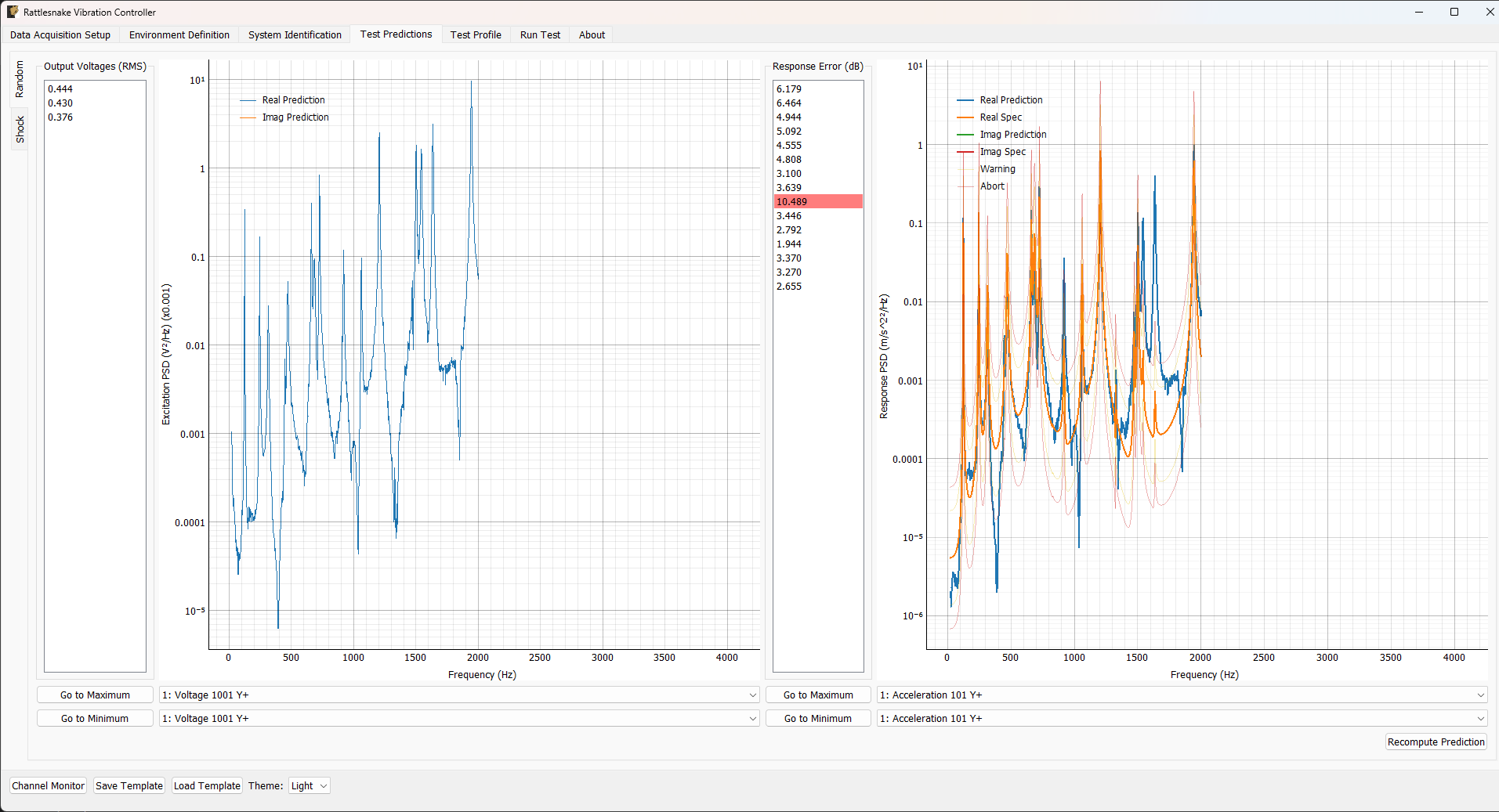
Figure 3.11:Test prediction tab showing the prediction for each environment on a separate subtab.
The Test Prediction tab will again have a subtab for each environment containing the test predictions for that environment. The prediction presented will vary with environment type, as each environment will generally compare predicted response back to the specification. A Chapter 12 environment will therefore make comparisons to a CPSD matrix while a Chapter 13 will make comparisons to time data. See the chapters in Part 3: Rattlesnake Environments for prediction specifics for each environment.
3.5Test Profiles
The Test Profile tab gives the user the ability to set up a test timeline for complex combined environments tests. The user can add a list of events that will be executed at certain times during the test. The tab will also display a graphical representation of the test timeline.
Events can be added or removed from the test timeline by clicking the Add Event or Remove Event buttons. Users can also load a series of events from or save a series of events to an Excel spreadsheet or CSV file.
For each event, the following parameters are defined:
Timestamp (s) The time in seconds after the timeline has started that the event will be executed.
Environment The environment in which the event will occur.
Operation The operation that will occur to the event. Each environment defines its own set of operations that can be executed through the test profile interface.
Data Any additional data that the operation requires. For example, if a “Set Test Level” event is chosen, the Data field should specify the value that the test level is set to.
Figure 3.12 shows an example of a test profile that ramps up the test level of environment Random from -6 to 0 dB, and then subsequently starts environment Shock.
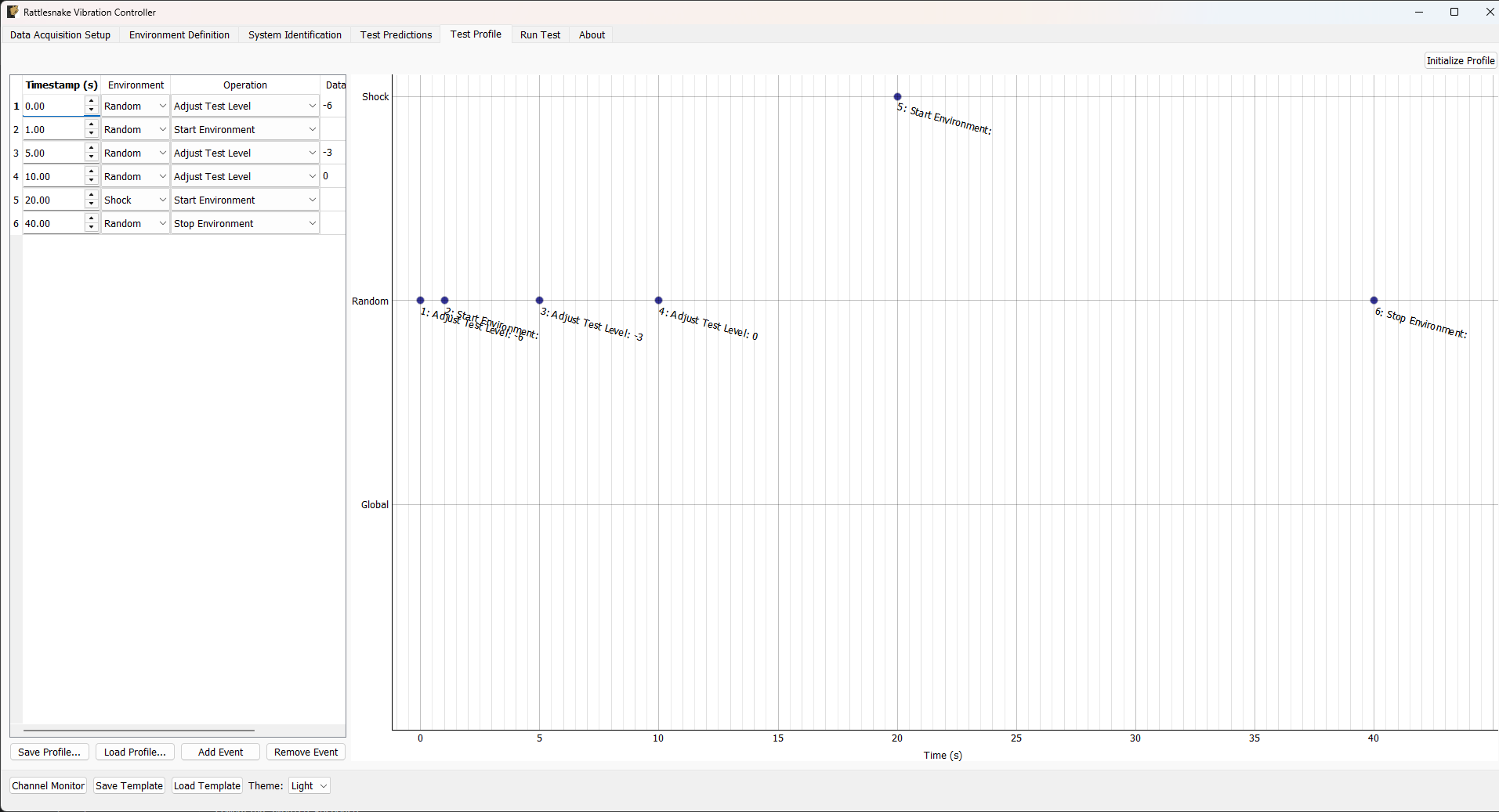
Figure 3.12:Example test profile showing a ramp up of test level for environment Random and subsequently starting environment Shock.
3.6Run Test
The Run Test tab is where Rattlesnake finally runs the test. This tab again has sub-tabs for the different environments in the test, however these sub-tabs will not be enabled until the data acquisition system is armed.
Rattlesnake gives the user many options to save data to the disk through a set of Radio buttons at the top of this tab. These options are:
No Streaming Do not save data to disk, just run the test.
Start Streaming from Test Profile Instruction Selecting this option allows data to be saved to disk after a “Global Start Streaming” event from the test profile is executed. This allows the user to fine tune at which point in the test data is acquired.
Start Streaming at Target Test Level Selecting this option starts streaming data when the selected environment hits its target test level. This can be useful if, for example in a random environment, the user wishes to start at a low level and slowly creep up to the target test level. If all data is saved, it might require a large amount of file space, so instead only the data at the test level of interest can be saved.
Start Streaming Immediately Saves all data from the time the first environment starts until the data acquisition system is disarmed.
Manually Start/Stop Streaming Allows the user to start and stop the measurement periodically throughout the test. A
Start Streamingbutton will appear when this option is selected. When clicked, the button will change toStop Streaming. Multiple data streams can be saved in a given test. These will be stored to separate variables in the output NetCDF4 file (see Section 3.7).
When streaming data, it is important to note that the software does not stop streaming until the data acquisition system is disarmed by pressing the Disarm Data Acquisition button. This is because for a combined-environments test, the environments may have down-time between them where no environment is running, and that data should still be saved.
The Run Test tab contains global Arm Data Acquisition and Disarm Data Acquisition buttons that start and stop the data acquisition system. When the data acquisition system is armed, the user can no longer change streaming options, and the sub-tabs for each environment are enabled. The user can then start or stop each environment manually using the Start Environment or Stop Environment buttons on each environment’s sub-tab. The sub-tab for each environment is described more thoroughly in Part 3: Rattlesnake Environments.
Alternatively, the user can start or stop the test profile by clicking on the Start Profile or Stop Profile buttons respectively. The profile capability also includes the option to switch the active environment sub-tab when an event is executed so the user can see the results. Note that the profile options only appear when a profile has been defined on the Test Profile tab.
Figure 3.13 shows an example Run Test tab with test profile events.
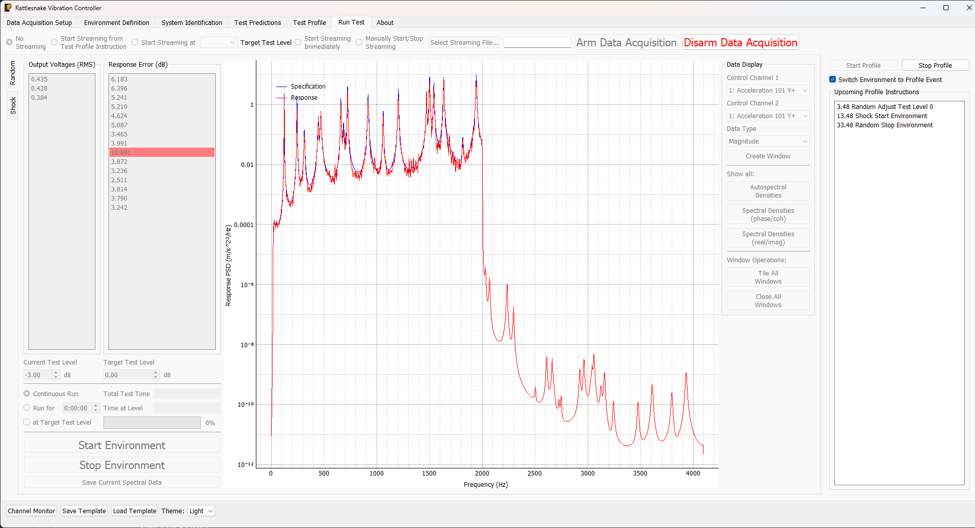
Figure 3.13:Run Test Tab.
3.7Rattlesnake Output Files
After streaming data is acquired, the user may wish to analyze or plot the data acquired for a given test report. Rattlesnake streams data to a self-documenting netCDF file 1, which can be read by multiple platforms. The output file is described as self-documenting because it contains all parameters necessary to reconstruct a given test using the Rattlesnake controller. Any parameter that is set by the user in the UI is stored to the netCDF file.
A full description of the netCDF file format is out of this document’s scope, but the important points are briefly described here. NetCDF files have a number of data structures.
Variables are multi-dimensional arrays of data.
Dimensions describe the axes of the variable arrays.
Attributes are used to store small data such as scalars or 1D arrays.
The NetCDF file content can be separated into different Groups, and each group can have its own variables, dimensions, and attributes.
The Rattlesnake output files contain the following data members:
3.7.1NetCDF Dimensions 
response_channelsThe number of response channels in a given testoutput_channelsThe number of output channels in a given testtime_samplesThe number of time samples measured in the file, this dimension can expand as more data is acquired.time_samples_XIf manual streaming is used and streaming is started multiple times, each subsequent stream will have thetime_samplesname with an underscore and appended number (e.g.time_samples_1,time_samples_2). This also occurs when streaming system identification data; the noise measurement is stored in a variable with dimensiontime_samplesand the system identification data is stored in a variable with dimensiontime_samples_1.num_environmentsThe total number of environments in the test
3.7.2NetCDF Attributes 
file_versionA version number of the software that the file was written for.sample_rateThe global sample rate of the data acquisition systemtime_per_writeThe amount of data put to the output hardware per write operation, in secondstime_to_readThe amount of data read from the acquisition hardware per read operation, in secondshardwareThe hardware index used for the test.0 -- National Instruments NI-DAQmx
1 -- HBK LAN-XI Open API
2 -- Data Physics Quattro
3 -- Data Physics 900 Series
4 -- Virtual Control defined by Exodus Modal Solution
5 -- Virtual Control defined by State Space Matrices
6 -- Virtual Control defined with a SDynPy System
hardware_fileThe path to the file used to define the Virtual test article, or the path to the external code library used by the data acquisition hardware. Otherwise, it will beNoneoutput_oversampleThe oversample used either due to sample rate restrictions on the data acquisition system, or due to oversampling the integration
3.7.3NetCDF Variables 
time_dataThe measured data from the test. Type: 64-bit float; Dimensions:response_channelsbytime_samplestime_data_XIf manual streaming is used and streaming is started multiple times, each subsequent stream will have thetime_dataname with an underscore and appended number (e.g.time_data_1,time_data_2). This also occurs when streaming system identification data; the noise measurement is stored in a variabletime_dataand the system identification data is stored in a variabletime_data_1; Dimensions:response_channelsbytime_samples_Xenvironment_namesThe name of each environment. Type: string; Dimensions:num_environmentsenvironment_active_channelsThe channels active in each environment. 1 if active, 0 if not. Type: 8-bit int; Dimensions:response_channelsnum_environments
3.7.4Channels Group 
The netCDF files from Rattlesnake store all channel information into a separate group called channels. Inside the channels group, there is a variable for each column of the channel table. See Section #sec:channel_table for more complete descriptions of each channel variable.
/channels/node_numberThe node number of each channel. Type: str; Dimensions:response_channels/channels/node_directionThe instrument direction of each channel. Type: str; Dimensions:response_channels/channels/commentThe commend for each channel. Type: str; Dimensions:response_channels/channels/serial_numberThe serial number of the instrument for each channel. Type: str; Dimensions:response_channels/channels/triax_dofThe sensor degree of freedom for each channel. Type: str; Dimensions:response_channels/channels/sensitivityThe sensitivity of the instrument for each channel. Type: str; Dimensions:response_channels/channels/unitThe engineering unit of the instrument for each channel. Type: str; Dimensions:response_channels/channels/makeThe manufacturer of the instrument for each channel. Type: str; Dimensions:response_channels/channels/modelThe model number or product name of the instrument for each channel. Type: str; Dimensions:response_channels/channels/expirationThe expiration date of the instrument’s calibration for each channel. Type: str; Dimensions:response_channels/channels/physical_deviceThe physical device that the instrument is connected to for each channel. Type: str; Dimensions:response_channels/channels/physical_channelThe channel in the physical device that the instrument is attached to for each channel. Type: str; Dimensions:response_channels/channels/channel_typeThe type of quantity that is measured by the channel. Type: str; Dimensions:response_channels/channels/minimum_valueThe minimum voltage that the channel can accept. Type: str; Dimensions:response_channels/channels/maximum_valueThe maximum voltage that the channel can accept. Type: str; Dimensions:response_channels/channels/couplingThe coupling type used by each channel (AC/DC/filter/etc.). Type: str; Dimensions:response_channels/channels/excitation_sourceThe excitation source for each channel, used to specify CCLD/ICP/IEPE. Type: str; Dimensions:response_channels/channels/excitationThe excitation current value used in the signal conditioning for each channel. Type: str; Dimensions:response_channels/channels/feedback_deviceThe device that the channel’s generator originates from if the channel is an output channel. Type: str; Dimensions:response_channels/channels/feedback_channelThe channel that the channel’s generator originates from if the channel is an output channel. Type: str; Dimensions:response_channels/channels/warning_levelThe warning level of each channel. Type: str; Dimensions:response_channels/channels/abort_levelThe abort level of each channel. Type: str; Dimensions:response_channels
3.7.5Environment Groups 
Environment-specific attributes, dimensions, and variables are also stored within a group corresponding to each environment. For example, in the case where there were two environments “Random” and “Shock”, parameters specific to environment “Random” would be stored within the group “Random” in the netCDF file, and similarly for “Shock”. See the chapters in Part 3: Rattlesnake Environments for more information on environment-specific parameters.
3.7.6Reading Rattlesnake Output Files using Python 
To read data from a netCDF using Python, it is recommended to use the netCDF4 Python package. This library is a dependency of Rattlesnake, so if the user is not running Rattlesnake via an executable, this package should already be installed in the user’s Python ecosystem.
netCDF4 provides a sleek Python interface into the data of a netCDF4 file. This section will assume the command import netCDF4 as nc4 was used to import the package, so nc4 is used as a shorter alias.
A netCDF4 dataset can be opened using the following command:
dataset = nc4.Dataset('path/to/netcdf4/file.nc4')after which all data can be accessed through the dataset object.
Attribute names can be queried using the dataset.ncattrs() function and the attribute values can be accessed directly from the dataset object using that name.
>>> dataset.ncattrs()
['file_version',
 'sample_rate',
 'time_per_write',
 'time_per_read',
 'hardware',
 'output_oversample',
 'hardware_file']

>>> dataset.sample_rate
8192
Dimensions can be accessed using the dataset.dimensions property, which gives a Python dict where the keys are the dimension names and the values are references to the dimension. The size of the dimension can be accessed using the size parameter in each dimension object.
>>> dataset.dimensions
{'response_channels': "<class 'netCDF4.Dimension'>": name = 'response_channels', size = 26,
 'output_channels': "<class 'netCDF4.Dimension'>": name = 'output_channels', size = 3,
 'time_samples': "<class 'netCDF4.Dimension'>" (unlimited): name = 'time_samples', size = 342016,
 'num_environments': "<class 'netCDF4.Dimension'>": name = 'num_environments', size = 2}

>>> dataset.dimensions['response_channels'].size
30
Variables can be accessed similarly to dimensions using the dataset.variables property. Variables have many properties that may be interesting to the users, including the netCDF dimensions that were used to size the variable (accessible with the dimensions parameter) or the actual shape of the array (accessible with the shape parameter). The data inside the dimension can be accessed by slicing or indexing the array, or simply passing it to a numpy array. Note that slicing or indexing the variable returns the data in a numpy masked array which allows data to potentially to be missing from the array. Rattlesnake does not use the missing data capabilities of the netCDF file, so data can safely be transformed directly to a regular numpy array.
>>> dataset.variables
{'time_data': <class 'netCDF4.Variable'>
 float64 time_data(response_channels, time_samples)
 unlimited dimensions: time_samples
 current shape = (26, 342016)
 filling on, default _FillValue of 9.969209968386869e+36 used,
 'environment_names': <class 'netCDF4.Variable'>
 vlen environment_names(num_environments)
 vlen data type: <class 'str'>
 unlimited dimensions:
 current shape = (2,),
 'environment_types': <class 'netCDF4.Variable'>
 int64 environment_types(num_environments)
 unlimited dimensions:
 current shape = (2,)
 filling on, default _FillValue of -9223372036854775806 used,
 'environment_active_channels': <class 'netCDF4.Variable'>
 int8 environment_active_channels(response_channels, num_environments)
 unlimited dimensions:
 current shape = (26, 2)
 filling on, default _FillValue of -127 ignored}

# Get the dimensions used by the variable
>>> dataset.variables['time_data'].dimensions
('response_channels', 'time_samples')

# Get the shape of the variable
>>> dataset.variables['time_data'].shape
(26, 342016)

# Access via slice returns a masked array
>>> dataset.variables['time_data'][0,0]
masked_array(data=0.,
             mask=False,
       fill_value=1e+20)

# Can pass directly to a numpy array to get the full variable data
>>> np.array(dataset.variables['time_data'])
array([[ 0.00000000e+00,  0.00000000e+00,  0.00000000e+00, ...,
        -9.34897708e-09, -3.00422105e-09,  4.85883640e-09],
       [ 0.00000000e+00,  0.00000000e+00,  0.00000000e+00, ...,
        -1.12773608e-08, -3.25183298e-09,  6.64041130e-09],
       [ 0.00000000e+00,  0.00000000e+00,  0.00000000e+00, ...,
         4.32735251e-08,  3.73648821e-08,  2.12970606e-08],
       ...,
       [ 0.00000000e+00,  0.00000000e+00,  0.00000000e+00, ...,
         0.00000000e+00,  0.00000000e+00,  0.00000000e+00],
       [ 0.00000000e+00,  0.00000000e+00,  0.00000000e+00, ...,
         0.00000000e+00,  0.00000000e+00,  0.00000000e+00],
       [ 0.00000000e+00,  0.00000000e+00,  0.00000000e+00, ...,
         0.00000000e+00,  0.00000000e+00,  0.00000000e+00]],
      shape=(26, 342016))
Group names in the netCDF dataset can be queried using dataset.groups, which returns a dictionary similar to the dimensions and variables. Groups can also be accessed by indexing the dataset directly with the group name. A group object can be treated exactly the same as the root-level dataset, and will have its own set of attributes, dimensions, and variables.
>>> dataset['channels'].variables['node_number']
<class 'netCDF4.Variable'>
vlen node_number(response_channels)
vlen data type: <class 'str'>
path = /channels
unlimited dimensions:
current shape = (26,)3.7.7Reading Rattlesnake Output Files using Matlab 
Matlab can also be used to read netCDF files from Rattlesnake. The Matlab ncdisp function can be used to quickly determine which parameters are in a file.
>>> ncdisp('path/to/netcdf/file.nc4')
Source:
           path/to/netcdf/file.nc4
Format:
           netcdf4
Global Attributes:
           file_version      = '3.0.0'
           sample_rate       = 8192
           time_per_write    = 0.25
           time_per_read     = 0.25
           hardware          = 5
           output_oversample = 10
           hardware_file     = 'path/to/hardware/file.npz'
Dimensions:
           response_channels = 26
           output_channels   = 3
           time_samples      = 342016 (UNLIMITED)
           num_environments  = 2
Variables:
    time_data
           Size:       342016x26
           Dimensions: time_samples,response_channels
           Datatype:   double
    environment_names
           Size:       2x1
           Dimensions: num_environments
           Datatype:   string
    environment_types
           Size:       2x1
           Dimensions: num_environments
           Datatype:   int64
    environment_active_channels
           Size:       2x26
           Dimensions: num_environments,response_channels
           Datatype:   int8
Groups:
    /channels/
        Variables:
            node_number
                   Size:       26x1
                   Dimensions: /response_channels
                   Datatype:   string
       .
       .
       .
Attributes, dimensions, and other metadata can be read into Matlab using the ncinfo function. Variables information must be read using the ncread function.
>>> finfo = ncinfo('path/to/netcdf/file.nc4')

finfo =

  struct with fields:

      Filename: 'C:\Users\dprohe\Documents\Local_Repositories\Rattlesnake_External\src\rattlesnake\examples\frame_wing\data\streaming_example.nc4'
          Name: '/'
    Dimensions: [1×4 struct]
     Variables: [1×4 struct]
    Attributes: [1×7 struct]
        Groups: [1×3 struct]
        Format: 'netcdf4'
     Datatypes: []

>>> finfo.Dimensions(1)

ans =

  struct with fields:

         Name: 'response_channels'
       Length: 26
    Unlimited: 0

>>> time_data = ncread('path/to/netcdf/file.nc4','time_data')
Variables within groups can be read by concatenating the group name with the variable name, similar to a file system.
>>> ncread('path/to/netcdf/file.nc4','channels/node_number')

ans =

  26×1 string array

    "101"
    "102"
    "103"
    "104"
    "105"
    "106"
    "107"
    "101"
    .
    .
    .
In older versions of Matlab, one issue that may be encountered is that string variables are unsupported. This means that the majority of the channel information cannot be read through the Matlab netCDF interface in these versions of Matlab. However, they can be read using the lower level h5read function. Recent versions of Matlab do not have this issue.
>>> ncread('path/to/netcdf/file.nc4','channels/node_number')
Error using netcdf.getVar (line 137)
12 is not a recognized netCDF datatype.

Error in internal.matlab.imagesci.nc/read (line 605)
                data = netcdf.getVar(gid, varid);

Error in ncread (line 66)
vardata = ncObj.read(varName, varargin{:});

>>> h5read(file,'/channels/node_number')

ans =

26x1 cell array3.8Saving and Loading Rattlesnake Tests
It can be tedious to set up a test from scratch each time a test is to be run, so Rattlesnake offers two ways to load test settings from files. Both of these approaches can be accessed by clicking the Load Template button on the main Rattlesnake UI, shown in Figure 3.14.
The first approach to loading a Rattlesnake test is to load in any output Rattlesnake netCDF file. Because Rattlesnake stores all of the metadata associated with a test to this file, Rattlesnake can simply load the metadata from the file to reconstruct that test. One must be careful with various file paths to ensure they are consistent if loading tests from a different computer or file system. For example, the path to a control law on one computer may not be the same path to that file on a different computer.
The second way to load a test is to load in an Excel spreadsheet “template” file. This file will include a worksheet for the channel table, the hardware, each environment, and the test profile. The template can be created by clicking the Save Template button on the main Rattlesnake UI, shown in Figure 3.14. Saving the template will populate it as much as possible with the content from the UI. Commonly missing in environments is the path to the specification file that should be loaded, as some environments do not save this data, and it would be tedious to enter a multidimensional array into a spreadsheeet. Once completed, this file can be loaded by clicking the Load Template button.

Figure 3.14:View of the Channel Monitor dialog box showing several channels that have reached the “warning” level (highlighted yellow) and one channel that has reached the “abort” level (highlighted red).
3.9Channel Monitor 
To aid with understanding the test levels and headroom available for the sensors in the test, a Channel Monitor is available where the levels are shown for each channel. The channel monitor is displayed by clicking on the Channel Monitor button on the lower left side of the UI. The display shows both an instantaneous level (green) as well as a running historical maximum (blue). If a channel reaches the Warning or Abort level, it will be flagged with a yellow or red tint, respectively. These warnings “latch”; once the level is reached, it will stay highlighted in the channel monitor until the Clear Alerts button is clicked. Figure 3.15 shows an example channel monitor.
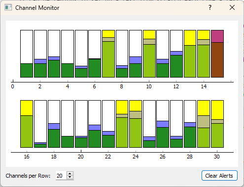
Figure 3.15:View of the Channel Monitor dialog box showing several channels that have reached the “warning” level (highlighted yellow) and one channel that has reached the “abort” level (highlighted red).
The aspect ratio of the Channel Monitor can be customized to different sizes modifying the Channels per Row.
3.10Example Problems
Learning to use Rattlesnake by reading the User’s Manual cover-to-cover is likely not the best way to start using Rattlesnake. The best way to learn how to use Rattlesnake is to start using it, and then to reference the User’s Manual when clarification is needed. This user’s manual contains multiple example problems in the chapters of Examples. New users are suggested to start with these example problems to gain experience and context with MIMO testing.
- Unidata. (2019). Network Comon Data Form (netCDF) version 4.4.1.1. Software. 10.5065/D6H70CW6