12Multiple Input/Multiple Output Random Vibration
The first environment implemented in the Rattlesnake controller was the MIMO Random Vibration environment. This environment aims to control the vibration response of a component to specified levels by creating output signals with the correct levels, coherence, and phase at each frequency line. The governing equation for MIMO Random Vibration is
where the CPSD matrix of the responses result from some signals exciting the structure represented by transfer function matrices . In a typical vibration control problem, the control system tries to compute the signal matrix that best reproduces the desired response .
12.1Specification Definition
The first step in defining a Random Vibration control problem is the definition of the vibration response that is desired. This vibration specification can be derived using various approaches, perhaps from test data from some environment test, predictions from a model, or derivations from a standard. Regardless of its source, the specification defines the response levels, coherence, and phase of each control channel at each frequency line in the test.
Rattlesnake accepts the specification in the form of a 3D array consisting of a complex CPSD matrix defined at each frequency line. Specification CPSD matrices can be loaded from Numpy *.npz files or Matlab *.mat files. For each of these files, Rattlesnake respects the natural dimension ordering of a dataset consisting of “stacks” of matrices that the specification can be visualized to be. For Matlab, which customarily uses the third dimension as the “stacking” dimension for 3D datasets, the specification dimensions should be where is the number of control channels and is the number of frequency lines. For Numpy/Python the more natural ordering is , essentially taking the last dimension of the Matlab array and moving it to the first dimension in the Numpy array. Both Matlab *.mat and Numpy *.npz files should contain the following data fields:
cpsd A (for
*.npzfiles) or (for*.matfiles) complex array containing the CPSD matrix at each frequency defined inf.f A array of frequencies corresponding to the frequency lines in the
CPSDmatrix.
For example, for a test consisting of three control channels has a given specification is defined from 10 Hz to 100 Hz with 2 Hz spacing, the variable f in the specification file would be length 46 and have values [10, 12, 14, ... 98, 100] and the variable cpsd would be size in a *.npz file or in a *.mat file.
The ordering of the rows and columns of the CPSD matrices defining the specification are the same order as the control channels in the Channel Table on the Data Acquisition Setup tab. This means that the first row and column of the CPSD matrix will correspond to the first channel that is selected as a control channel in the Control Channels list on the Environment Definitions tab. The second row and column to the second channel selected as a control channel, and so on. Note that if Control transformations are specified, then the first row and column of the specification will correspond to the first virtual control channel, which is the first row of the control transformation matrix. The second row and column will correspond to the second virtual control channel.
The specification is defined in units of where is the engineering unit specified by the Engineering Unit column of the channel table for the control channels.
Rattlesnake MIMO Random Vibration specification files can also contain optional warning and abort limits. Note that these limits only operate on the APSD portion (i.e. the diagonal) of the CPSD matrices. It is not currently possible to set a limit based on, for example, the coherence between two channels in Rattlesnake. These are defined in the specification files in fields:
warning_upper A (for
*.npzfiles) or (for*.matfiles) array containing an upper warning level at each frequency defined inffor each control channel.warning_lower A (for
*.npzfiles) or (for*.matfiles) array containing a lower warning level at each frequency defined inffor each control channel.abort_upper A (for
*.npzfiles) or (for*.matfiles) array containing an upper abort level at each frequency defined inffor each control channel.abort_lower A (for
*.npzfiles) or (for*.matfiles) array containing a lower abort level at each frequency defined inffor each control channel.
Any combination of the above fields can be specified. For example, a lower limit can be defined without an equivalent upper limit. An abort limit can be defined without a warning limit. However, if the field is defined in the specification file, it must have the correct shape, which means that the limit must be defined for all frequency lines and for all control channels. If a user does not want to limit on specific frequency ranges or specific channels, the limit can be set to a value of NaN. Rattlesnake will ignore portions of the limit specifications that contain NaN values.
Throughout the MIMO Random Vibration environment, channels will be flagged as yellow if they cross a warning limit, and flagged as red if they cross an abort limit. Additionally, if the Allow Automatic Aborts? checkbox is checked on the Environment Definition tab, the environment will automatically stop if the abort limit is crossed.
12.2Defining the MIMO Random Vibration Environment in Rattlesnake
In addition to the specification, there are a number of signal processing parameters that are used by the MIMO Random Vibration environment. These, along with the specification, are defined on the Environment Definition tab in the Rattlesnake controller on a sub-tab corresponding to a MIMO Random Vibration environment. Figure 12.1 shows a MIMO Random Vibration sub-tab. The following subsections describe the parameters that can be specified, as well as their effects on the analysis.
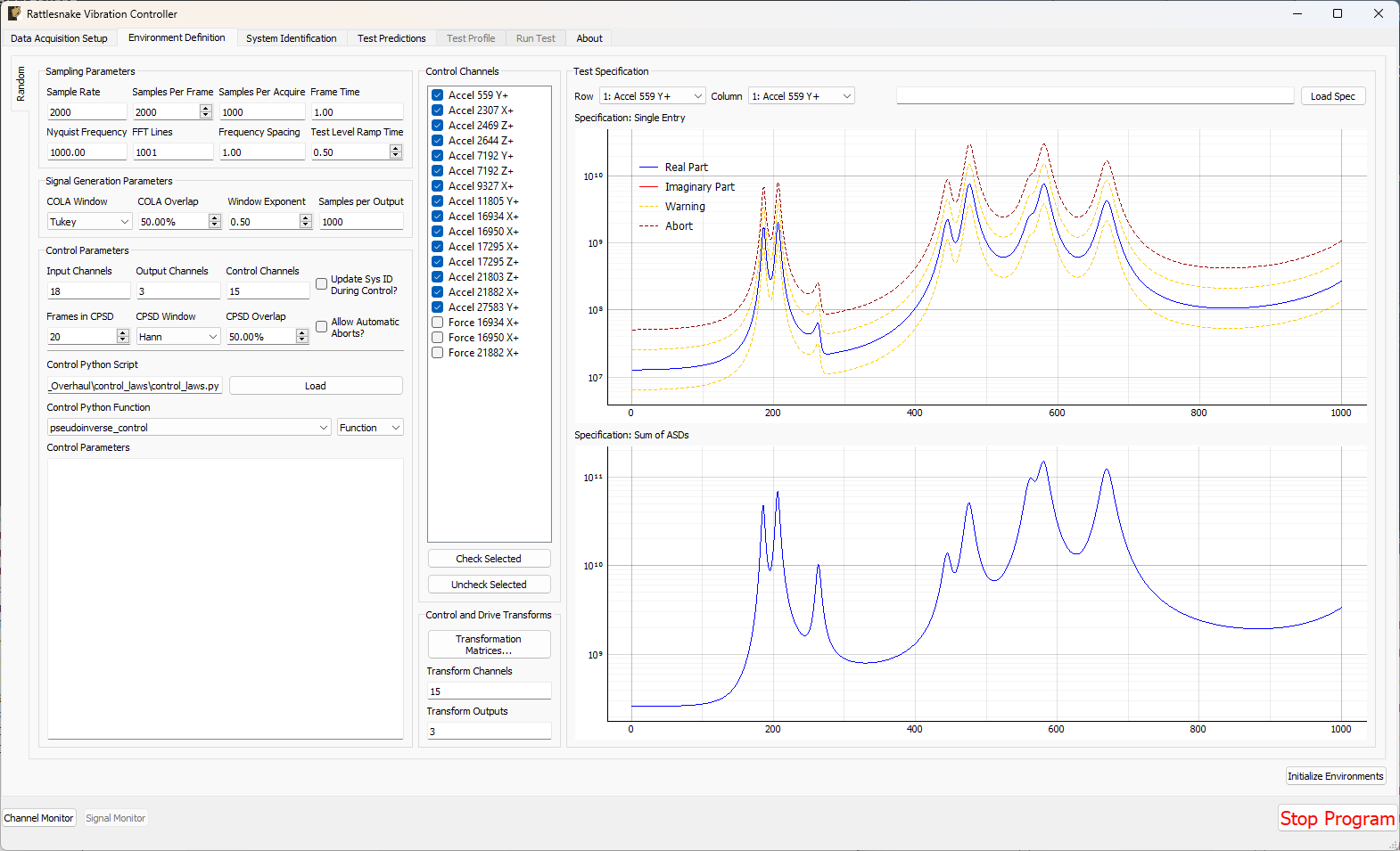
Figure 12.1:GUI used to define a MIMO Random Vibration environment.
12.2.1Sampling Parameters
The Sampling Parameters Settings section of the MIMO Random Vibration definition sub-tab consists of the following parameters:
Sample Rate Sample rate in samples per second of the data acquisition hardware, for display only. This is a global parameter and must be set in the Data Acquisition Setup tab.
Samples per Frame Samples per measurement frame in the controller. The measurement frame is the “block” of data upon which the signal processing will be performed. This value will determine the window size. A larger value will result in more frequency lines in the FFT analysis. This need not correspond to the read or write size in the data acquisition system.
Samples per Acquire Number of samples that the control process processes at a time. This will be equal to the Samples per Frame * (1 - Overlap Percentage / 100). This need not correspond to the read or write size of the data acquisition system as the control process acquisition is buffered.
Frame Time Time to acquire each measurement frame in seconds. This is the Samples per Frame divided by the Sample Rate.
Nyquist Frequency The Nyquist Frequency is the highest frequency that can be analyzed using frequency domain techniques. It is the Sample Rate / 2.
FFT Lines The number of frequency lines in the Fast Fourier Transform output, which is the number of frequency lines that will be in the Transfer Function and CPSD matrices.
Frequency Spacing The frequency resolution of the measurement, computed by 1/Frame Time.
Test Level Ramp Time Time in seconds that the controller takes to change the test level. The test level is changed smoothly to prevent damaging the excitation hardware or part under test. Larger numbers will result in a more smooth transition between test levels, while smaller numbers will make the test level change more quickly.
12.2.2Signal Generation Parameters
The Sampling Parameters Settings section of the MIMO Random Vibration definition sub-tab consists of the following parameters:
COLA Window Window function to use when performing the Constant Overlap and Add to combine time realizations into a continuous signal. A Hann window is limited to 50% overlap. Tukey windows can have variable overlap.
COLA Overlap Percentage overlap between frames that are assembled using the Constant Overlap and Add
Window Exponent Exponent that the window function is raised to. This should typically be 0.5 to ensure a constant variance in the signal. Don’t change this value unless you know what you’re doing.
Samples per Output Number of new samples generated by each realization taking into account the overlap with the previous realization.
Sigma Clipping Number of standard deviations to include in the output signal. A value of 5 corresponds to effectively no clipping. A value of 3 is commonly used to reduce peak displacement. Setting this value too low will result in loss of dynamic range and non-gaussian output signals.
12.2.3CPSD Parameters
The CPSD Parameters Settings section of the MIMO Random Vibration Controller sub-tab consists of the following parameters:
Frames in CPSD Number of measurement frames to use when computing CPSD matrices. Fewer frames will result in more responsive control. More frames will result in better averaging and noise rejection.
CPSD Window Window function to use when computing CPSDs.
CPSD Overlap Percentage overlap between measurements when constructing CPSDs.
12.2.4Tolerances and Options
The Tolerances Settings and Options Settings sections of the MIMO Random Vibration Controller sub-tab consists of the following parameters:
Frequency Lines Out Percentage of control frequency lines that can fall outside of limits before triggering warnings/aborts.
Allow Automatic Aborts? If checked, the controller will automatically abort if the abort level in the specification is hit.
Update Sys ID During Control? Checking this box will allow the controller to continually update the system identification to perhaps get a better control for nonlinear structures. Use with caution! If, for example, a shaker becomes disconnected, the controller will see the system identification between that shaker and the control channels become very small, and it will therefore try to push the shaker harder to make up for the poor transfer function, so the problem could explode.
12.2.5Control Parameters
The Control Parameters Settings section of the MIMO Random Vibration definition sub-tab contains functionality for loading in custom control laws. See Section 12.7 for information on defining a custom control law.
Load Opens a file dialog to load in a Python script containing the control law.
Control Python Script Python script used to specify the control law.
Control Python Function Selects the function, generator function, or class in the Python script to use as the control law.
Control Type Select if the selected control law is a Function, Generator, Class, or Interactive Class. This should be detected automatically by inspection; users should not have to adjust this.
Control Parameters Any additional parameters needed by the control law are entered in this text box. It is up to the control law to prescribe what is needed to be defined in this box. The data entered into this box will be passed to the control law as a string to the “extra_parameters” argument. Control laws should parse this string to extract needed information.
12.2.6Control Channels
The Control Channels Settings list allows users to select the channels in the test that will be used by the environment to perform control calculations. These are the channels that will match the rows and columns of the specification file.
Control Channels Channels that are checked will be used as the control channels for this environment. The control channels should be ordered in the specification the same way they are ordered in this list. For example, the first row and column of the specification CPSD matrix will correspond to the first checked channel in this list.
Check Selected When clicked, any selected channels in the Control Channels list will be checked, and therefore used as control channels in the environment.
Uncheck Selected When clicked, any selected channels in the Control Channels list will be unchecked, and therefore not used as control channels in the environment.
12.2.7Channel I/O
The Channel I/O Settings section of the MIMO Random Vibration definition sub-tab consists of the following displays:
Input Channels A display showing the total number of physical channels this environment is measuring, including excitation channels and control channels.
Output Channels A display showing the total number of physical channels this environment is outputting to excitation devices such as vibration shakers.
Control Channels A display showing the total number of physical channels this environment is controlling to.
12.2.8Control and Drive Transforms
The Control and Drive Transforms Settings section of the MIMO Random Vibration definition sub-tab consists of the following parameters:
Transformation Matrices... Open the transformation matrix dialog to allow specification of transformations to virtual control or virtual excitation channels.
Transform Controls A display showing the number of virtual control channels in the environment due to transformation matrices applied to the physical control channels.
Transform Outputs A display showing the number of virtual excitation channels in the environment due to transformation matrices applied to the physical excitation channels.
Note that if transformation matrices are defined, the number of control channels ends up being the number of rows of the Response Transformation Matrix, rather than the number of physical control channels. The number of physical control channels will be equal to the number of columns of the transformation matrix. The number of rows and columns of the specification loaded should be equal to the number of rows in the transformation.
See Section 12.8 for more information on specifying transformation matrices.
12.2.9Test Specification
The test specification is loaded into the environment in the Test Specification Settings section of the MIMO Random Vibration definition:
Load Spec When clicked, opens a file dialog box to select a specification file to load.
Row Select the row of the CPSD matrix to visualize in the Specification: Single Entry plot.
Column Select the column of the CPSD matrix to visualize in the Specification: Single Entry plot.
Specification File Name File name of the loaded specification
Specification: Single Entry Displays a single entry in the specification CPSD matrix. If an off-diagonal value is selected, both real and imaginary parts will be shown. If warning and abort limits exist in the specification, these will also be shown.
Specification: Sum of ASDs Displays the trace (or sum of diagonals) of the CPSD matrix to give an overview of the frequency content in the specification.
12.3System Identification for the MIMO Random Vibration Environment
When all environments are defined and the Initialize Environments button is pressed, Rattlesnake will proceed to the next phase of the test, which is defined on the System Identification tab.
MIMO Random Vibration requires a system identification phase to compute the matrices used in the control calculations of equation (12.1). Figure 12.2 shows the GUI used to perform this phase of the test.
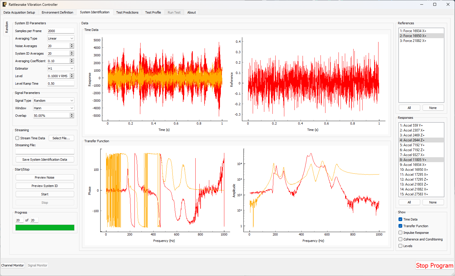
Figure 12.2:System identification GUI used by the MIMO Random Vibration environment.
Rattlesnake’s system identification phase will start with a noise floor check, where the data acquisition records data on all the channels without specifying an output signal. After the noise floor is computed, the system identification phase will play out the specified signals to the excitation devices, and transfer functions will be computed using the responses of the control channels to those excitation signals. Section 3.4 describes the System Identification tab and its various parameters and capabilities.
12.4Test Predictions for the MIMO Random Vibration Environment
Once the system identification is performed, a test prediction will be performed and results displayed on the Test Predictions tab, shown in Figure 12.3. This is meant to give the user an idea of the test feasibility. The left side of the window displays excitation information, including RMS signal levels required as well as the excitation spectra expected. The right side of the window displays the predicted responses compared to the specification as well as the predicted RMS dB error. This figure will also show any abort or warning limits imposed. Channels will be highlighted in yellow if they cross a warning level and will be highlighted in red if they cross an abort level. For example in the test in Figure 12.3, all channels are predicted to cross the warning threshold, and a handful are predicted to cross the abort threshold.
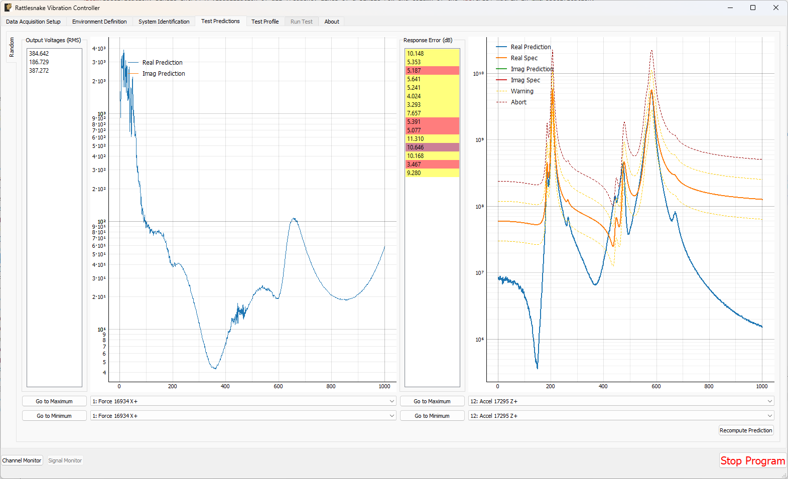
Figure 12.3:Test prediction GUI which gives the user some idea of the test feasibility.
In the Output Voltages (RMS) section of the window:
Output Voltage (RMS) RMS Voltage predicted for each excitation channel
Excitation Display Plot Shows the specified portion of the CPSD matrix. If an off-diagonal term is selected, both real and imaginary parts will be plotted.
Go to Maximum Excitation Shows the excitation channel with the largest voltage
Go to Minimum Excitation Shows the excitation channel with the smallest voltage
Excitation CPSD Row Channel Select the row of the excitation CPSD matrix to visualize
Excitation CPSD Column Channel Select the column of the excitation CPSD matrix to visualize
In the Response Error (dB) section of the window:
Response Error (dB) RMS dB error predicted at each control channel. Channels will be highlighted yellow if they hit a warning limit and red if they hit an abort limit. Double clicking on an item will show its response prediction.
Response Prediction Display Plot Shows the specified portion of the response CPSD matrix predicted using the computed excitation CPSD and system identification information compared to the specification. If an off-diagonal term is selected, both real and imaginary parts will be plotted.
Go to Maximum Response Error Show the control channel prediction with the largest predicted error
Go to Minimum Response Error Show the control channel prediction with the smallest predicted error
Response CPSD Row Channel Select the row of the response CPSD matrix to visualize
Response CPSD Column Channel Select the column of the response CPSD matrix to visualize
Clicking the Recompute Prediction button will run the control law again. It will use the previous prediction as if it were measured data, so closed loop control laws which operate on previous data may update their excitation and predictions.
Recompute Prediction Click to recompute the prediction by running the control law again.
12.5Running the MIMO Random Vibration Environment
The MIMO Random Vibration environment is then run on the Run Test tab of the controller.
With the data acquisition system armed, the environment can be started manually with the Start Environment button. Once running, it can be stopped manually with the Stop Environment button. With the data acquisition system armed and the environment running, the GUI looks like Figure 12.4.
Figure 12.4:GUI for running the MIMO Random Vibration environment.
There are various operations that can be performed when setting up and running the MIMO Random Vibration environment, and many visualization operations as well.
12.5.1Test Level
Two test levels exist in the MIMO Random Vibration Environment. The Current Test Level specifies the current level of the control in decibels relative to the specification level, which is 0 dB. Note that all data and visualizations on the Run Test window are scaled back to full level, so users should not be surprised if for example the values reported in the Output Voltages (RMS) table do not change significantly with test level. See Section 12.9 for more information on this implementation detail.
The second test level is the Target Test Level. This option can be used to specify a level at which data starts streaming to the disk if the user does not wish to save low level data. Additionally, the controller can be made to stop controlling automatically after a certain time at the target test level. This is done to ensure that the controller does not spend too much time at a level that could eventually damage a part.
Current Test Level Current test level in dB. 0 dB is the actual test level from the specification.
Target Test Level Target test level in dB. This can be used to automatically trigger streaming or used to stop the controller after a specified amount of time.
12.5.2Test Timing
The MIMO Random Vibration environment has multiple options for test timing. If Continuous Run is selected, the environment will continue until it is manually stopped. A specific run time can be specified using the Run for h:mm:ss option and specifying a time in the h:mm:ss selector. The at Target Test Level checkbox specifies whether or not to activate the timer at any test level or only when the test is at the target test level.
The MIMO Random Vibration environment will constantly update the Total Test Time and Time At Level time displays when the environment is active. A progress bar will be displayed when the controller is set to only run for a specified time. When the progress bar reaches 100%, the environment will shut down automatically.
Continuous Run Run the environment until it is manually stopped.
Run for (timed run) Run the environment for a specified amount of time
Run Time Amount of time that the environment will run for.
at Target Test Level If checked, the timer will only run when the test is at the target test level.
Total Test Time Total time that the environment has been running for at any level.
Time at Level Time that the environment has been running at the current test level.
Environment Progress When the bar reaches 100%, the environment will stop automatically. Will not be active during a continuous run.
12.5.3Starting and Stopping the Environment
When the run timing and test levels are configured to the user’s liking, the environment can be started manually with the Start Environment button. The environment will stop automatically if the run is timed; however, users can manually stop the environment by clicking on the Stop Environment button. While the environment is running, certain portions of the GUI will be disabled.
Start Environment Starts the environment controlling to the specification.
Stop Environment Stops the environment manually
12.5.4Test Metrics and Visualizations
The MIMO Random Vibration environment displays a number of global metrics to help evaluate the success of a test. RMS signal voltage values are displayed in the Output Voltages (RMS) table. RMS dB errors for each control channel are displayed in the Response Error (dB) table. These errors will also be colored yellow or red if the given channel is crossing a warning or abort level. If an abort level is reached and the Allow Automatic Aborts? option is selected on the Environment Definition page, then the environment will shut down automatically.
The Run Test tab for the MIMO Random Vibration environment displays the sum of APSD functions of the response CPSD matrix compared to the sum of APSD functions of the specification in a large plot in the middle of the main window, which can be seen in Figure 12.4. This can be considered an “Average” response level for the test compared to the “Average” specification level.
Output Voltages (RMS) Current excitation voltages being output from the controller.
Response Error (dB) Current control RMS dB error. Double clicking on an item will open up a window showing that channel’s magnitude. Channels will be highlighted yellow if they hit a warning limit and red if they hit an abort limit.
Sum of ASDs Display This plot shows the trace of the response CPSD matrix compared to the specification. This is essentially an “average” quantity, and individual channels may be higher or lower at each frequency line.
To interrogate specific channels, the Data Display section of the Run Test window offers several options. The row and column of the CPSD matrix can be selected using Control Channel 1 and Control Channel 2 selectors. The Data Type of the plot can be specified as Magnitude, Phase, Coherence, Real, or Imaginary. Pressing the Create Window button then creates the specified plot.
Control Channel 1 Row of the CPSD matrix to create a window for.
Control Channel 2 Column of the CPSD matrix to create a window for
Data Type Data type to display on the new visualization window.
Create Window Creates a new window to visualize the response of a given entry in the CPSD matrix with Control Channel 1 and Control Channel 2 specifying the row and column of the CPSD matrix, and Data Type specifying how the channel is displayed.
Some convenience operations are also included to visualize all channels. In the Show all: section, pressing the Autospectral Densities button will bring up one window per control channel and display the APSD function for each. Pressing the Spectral Densities (phase/coh) or Spectral Densities (real/imag) buttons will attempt to display the entire CPSD matrix, displaying either the phase and coherence or real and imaginary parts in the upper and lower triangular portions of the matrix.
Show All Autospectral Densities Show Autospectral Densities (ASDs) for all control channels. This will create a window for every channel in the test.
Show All Spectral Densities (phase/coh) Show the entire CPSD matrix. This will show Autospectral Densities on the diagonal, and phase and coherence on the off-diagonals.
Show All Spectral Densities (real/imag) Show the entire CPSD matrix. This will show Autospectral Densities on the diagonal, and real and imaginary parts on the off-diagonals.
Figure 12.5 shows an example displaying the full CPSD matrix with coherence and phase for a test with six control degrees of freedom.
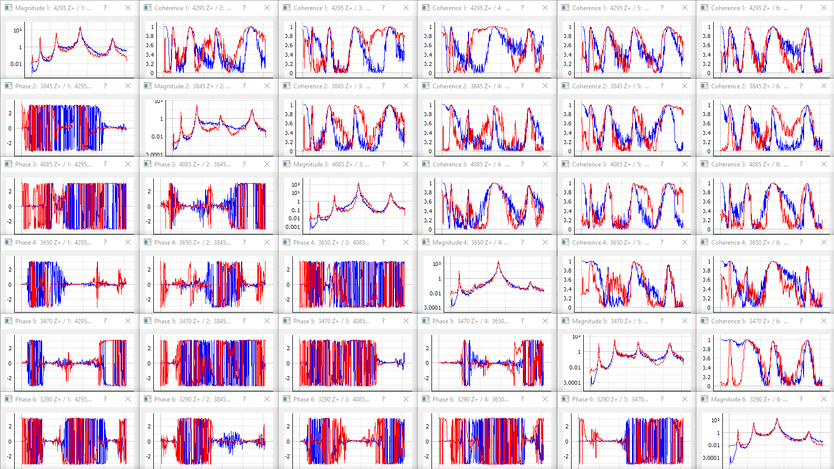
Figure 12.5:Visualizing individual channels (magnitude, coherence, and phase).
If a specification has warning and abort limits defined, these will also be plotted, as shown in Figure 12.6. Only APSD magnitude plots will show the warning and abort levels.
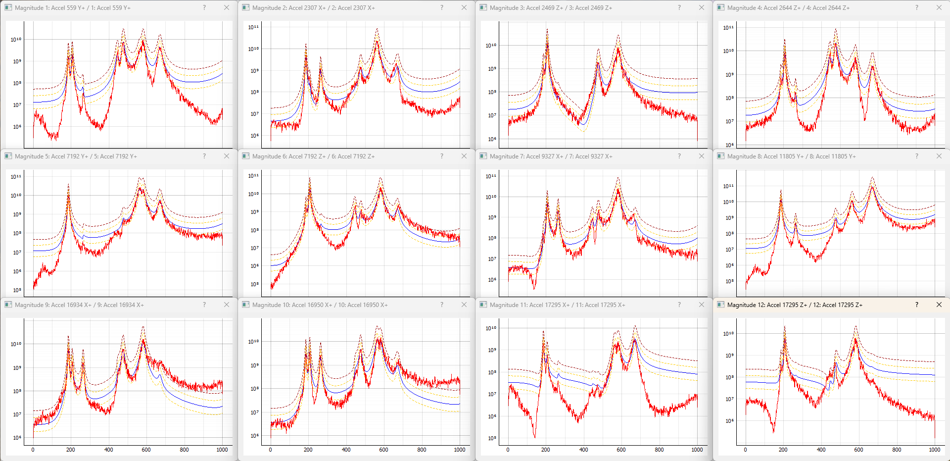
Figure 12.6:Figure showing the APSD data for each channel, as well as the warning and abort limits.
Further convenience operations are available in the Window Operations: section. Pressing Tile All Windows will rearrange all channel windows neatly across the screen. Pressing Close All Windows will close all open channel windows.
Tile All Windows Tiles all windows over the main monitor
Close All Windows Closes all visualization windows
12.5.5Saving Data from the MIMO Random Environment
Time data can be saved from the MIMO random vibration environment through Rattlesnake’s streaming functionality, described in Section 3.7.
Users can also directly write the spectral data from the environment to a file by clicking the Save Current Spectral Data button. This will also result in a netCDF file, however the fields will be slightly different. This is described more fully in Section 12.6.
Save Current Spectral Data Saves current spectral data to a NetCDF4 file.
12.6Output NetCDF File Structure
When Rattlesnake streams time data to a netCDF file, environment-specific parameters are stored in a netCDF group with the same name as the environment name. Similar to the root netCDF structure described in Section 3.8, this group will have its own attributes, dimensions, and variables, which are described here.
12.6.1NetCDF Dimensions
fft_lines The number of frequency lines in the FFT.
two A dimension of size 2, which is required for the warning and abort variables (there are two limits, upper and lower).
specification_channels The number of channels defined in the specification provided to the MIMO Random Vibration environment.
response_transformation_rows The number of rows in the response channel transformation (See Section 12.8). This is not defined if no response transformation is used.
response_transformation_cols The number of columns in the response channel transformation (See Section 12.8). This is not defined if no response transformation is used.
reference_transformation_rows The number of rows in the output transformation (See Section 12.8). This is not defined if no output transformation is used.
reference_transformation_cols The number of columns in the output transformation (See Section 12.8). This is not defined if no output transformation is used.
control_channels The number of physical channels used for control. Note that this may be different from the
specification_channelsdue to the presence of a transformation matrix.
12.6.2NetCDF Attributes
sysid_frame_size The number of samples per measurement frame in the system identification
sysid_averaging_type The type of averaging used in the system identification, linear or exponential
sysid_noise_averages The number of measurement frames acquired for the noise floor calculation
sysid_averages The number of measurement frames acquired for the system identification calculation
sysid_exponential_averaging_coefficient The weighting coefficient used for new frames in the exponential averaging scheme
sysid_estimator The FRF estimator used to compute the transfer functions during the system identification
sysid_level The level used by the system identification in volts RMS.
sysid_level_ramp_time The time to ramp up to the test level when starting and ramp back to zero when stopping the system identification
sysid_signal_type The signal type used by the system identification
sysid_window The window function applied to the time data during the system identification
sysid_overlap The overlap fraction between measurement frames used for system identification
sysid_burst_on The fraction of a measurement frame that a burst is active for burst random excitation during system identification
sysid_pretrigger The fraction of a measurement used as a pre-trigger for burst random excitation during system identification
sysid_burst_ramp_fraction The fraction of a measurement frame used to ramp the burst up to full level and back to zero
samples_per_frame The number of samples per measurement frame used in the FFT
test_level_ramp_time The time to ramp between test levels
cpsd_overlap The percentage overlap used when computing FRF and CPSD matrices
update_tf_during_control 1 if transfer functions were updated during control, 0 otherwise
cola_window The window function used by the COLA process
cola_overlap The overlap between realizations of excitation signals used during the COLA process
cola_window_exponent The exponent on the COLA window function
frames_in_cpsd The number of frames used to compute CPSD matrices
cpsd_window The window function used to compute CPSD matrices
control_python_script The path to the Python script used to control the MIMO Random Vibration environment
control_python_function The function (or class or generator function) in the Python script used to control the MIMO Random Vibration environment
control_python_function_type The type of the object used for the control law (function, generator, or class)
control_python_function_parameters The extra parameters passed to the control law.
12.6.3NetCDF Variables
specification_frequency_lines The frequency values in the specification associated with each frequency line. Type: 64-bit float; Dimensions:
fft_linesspecification_cpsd_matrix_real The real part of the MIMO Random Vibration specification. NetCDF files cannot handle complex data types so real and imaginary parts are split into two variables. Type: 64-bit float; Dimensions:
fft_linesspecification_channelsspecification_channelsspecification_cpsd_matrix_imag The imaginary part of the MIMO Random Vibration specification. NetCDF files cannot handle complex data types so real and imaginary parts are split into two variables. Type: 64-bit float; Dimensions:
fft_linesspecification_channelsspecification_channelsspecification_warning_matrix The data used to define the warning limits in the specification. The first index in the first dimension defines the lower limit, and the second index in the first dimension defines the upper limit. Type: 64-bit float; Dimensions:
twospecification_channelsspecification_abort_matrix The data used to define the abort limits in the specification. The first index in the first dimension defines the lower limit, and the second index in the first dimension defines the upper limit. Type: 64-bit float; Dimensions:
twospecification_channelsresponse_transformation_matrix The response transformation matrix (See Section 12.8). This is not defined if no response transformation is used. Type: 64-bit float; Dimensions:
response_transformation_rowsresponse_transformation_colsoutput_transformation_matrix The output transformation matrix (See Section 12.8). This is not defined if no output transformation is used. Type: 64-bit float; Dimensions:
output_transformation_rowsoutput_transformation_colscontrol_channel_indices The indices of the active control channels in the environment. Type: 32-bit int; Dimensions:
control_channels
12.6.4Saving Spectral Data
In addition to time streaming, Rattlesnake’s MIMO Random Vibration environment can also save the current realization of spectral data directly to the disk by clicking the Save Current Spectral Data button. The spectral data is stored in a NetCDF file similar to the time streaming data; however, it has additional dimensions and variables to store the spectral data.
The single additional dimension is:
drive_channels The number of drive channels active in the environment.
There are also several additional variables to store the spectral data:
frf_data_real The real part of the most recently computed value for the transfer functions between the excitation signals and the control response signals. NetCDF files cannot handle complex data types so real and imaginary parts are split into two variables. Type: 64-bit float; Dimensions:
fft_linesspecification_channelsdrive_channelsfrf_data_imag The imaginary part of the most recently computed value for the transfer functions between the excitation signals and the control response signals. NetCDF files cannot handle complex data types so real and imaginary parts are split into two variables. Type: 64-bit float; Dimensions:
fft_linesspecification_channelsdrive_channelsfrf_coherence The multiple coherence of the control channels computed during the test. Type: 64-bit float; Dimensions:
fft_linesspecification_channelsresponse_cpsd_real The real part of the most recently computed value for the CPSD matrix at the control channels. NetCDF files cannot handle complex data types so real and imaginary parts are split into two variables. Type: 64-bit float; Dimensions:
fft_linesspecification_channelsspecification_channelsresponse_cpsd_imag The imaginary part of the most recently computed value for the CPSD matrix at the control channels. NetCDF files cannot handle complex data types so real and imaginary parts are split into two variables. Type: 64-bit float; Dimensions:
fft_linesspecification_channelsspecification_channelsdrive_cpsd_real The real part of the most recently computed value for the CPSD matrix at the excitation channels. NetCDF files cannot handle complex data types so real and imaginary parts are split into two variables. Type: 64-bit float; Dimensions:
fft_linesdrive_channelsdrive_channelsdrive_cpsd_imag The imaginary part of the most recently computed value for the CPSD matrix at the excitation channels. NetCDF files cannot handle complex data types so real and imaginary parts are split into two variables. Type: 64-bit float; Dimensions:
fft_linesdrive_channelsdrive_channelsresponse_noise_cpsd_real The real part of the CPSD matrix at the control channels during the noise floor measurement that occurred during system identification. NetCDF files cannot handle complex data types so real and imaginary parts are split into two variables. Type: 64-bit float; Dimensions:
fft_linesspecification_channelsspecification_channelsresponse_noise_cpsd_imag The imaginary part of the CPSD matrix at the control channels during the noise floor measurement that occurred during system identification. NetCDF files cannot handle complex data types so real and imaginary parts are split into two variables. Type: 64-bit float; Dimensions:
fft_linesspecification_channelsspecification_channelsdrive_noise_cpsd_real The real part of the CPSD matrix at the excitation channels during the noise floor measurement that occurred during system identification. NetCDF files cannot handle complex data types so real and imaginary parts are split into two variables. Type: 64-bit float; Dimensions:
fft_linesdrive_channelsdrive_channelsdrive_noise_cpsd_imag The imaginary part of the CPSD matrix at the excitation channels during the noise floor measurement that occurred during system identification. NetCDF files cannot handle complex data types so real and imaginary parts are split into two variables. Type: 64-bit float; Dimensions:
fft_linesdrive_channelsdrive_channels
12.7Writing a Custom Control Law
The flexibility of the Rattlesnake framework is highlighted by the ease in which users can implement and iterate on their own ideas. For the MIMO Random Vibration control type, users can implement custom control laws using a custom Python function, or alternatively a generator function or class which allow state to be maintained between function calls. This section will provide instructions and examples for implementing a custom control law.
The controller will provide various data types to the control law functions which are:
specification-- The target CPSD matrix for the control channels; complex 3D array ()warning_levels-- The warning levels provided with the specification; complex 2D array ()abort_levels-- The abort levels provided with the specification; complex 2D array ()transfer_function-- The current estimate of the transfer function between the control responses and the excitation voltages; complex 3D array ()noise_response_cpsd-- The levels and correlation of the noise floor measurement on the control channels obtained during system identification; complex 3D array ()noise_reference_cpsd-- The levels and correlation of the noise floor measurement on the excitation channels obtained during system identification; complex 3D array ()sysid_response_cpsd-- The levels and correlation of the control channels obtained during system identification; complex 3D array ()sysid_reference_cpsd-- The levels and correlation of the noise floor measurement on the excitation channels obtained during system identification; complex 3D array ()multiple_coherence-- The multiple coherence for each control channel; real 2D array ()frames-- The number of measurement frames acquired so far, used to compute various parameters in the control law. This can be compared tototal_framesto determine if a full set of measurement frames has been acquired, or if the estimation of the various parameters could improve with continued averaging; scalar integertotal_frames-- The total number of frames used to compute the CPSD and FRF matrices; scalar integerextra_parameters-- Extra parameters provided to the controller. The control law can parse this value to allow extra arguments to be passed to the control law; stringlast_response_cpsd-- The most recent control CPSD, which can be used for error-based control; complex 3D array ()last_output_cpsd-- The most recent excitation CPSD, which can be used for drive-based control; complex 3D array ()
where size is the number of frequency lines, is the number of control channels, and is the number of output signals. Note that the values passed into the function may be defined using arbitrary variable names (e.g. transfer_function may be instead called H, or specification may be instead called spec or Syy); however, the order of the variables passed into each function will always be consistent.
12.7.1Defining a control law using a Python function
Python functions are the simplest approach to define a custom control law that can be used with the Rattlesnake software; however, they are limited in that a function’s state is completely lost when a function returns. Still, they can be used to implement relatively complex control laws as long as no state persistence is required.
A Python function used to define a MIMO Random Vibration control law in Rattlesnake would have the following general structure within a Python script.
# Any module imports, initialization code, or helper functions would go here

# Now we define the control law.  It always receives the same arguments from the controller.
def control_law(specification, # Specifications
                warning_levels, # Warning levels
                abort_levels, # Abort Levels
                transfer_function,  # Transfer Functions
                noise_response_cpsd,  # Noise levels and correlation
                noise_reference_cpsd, # from the system identification
                sysid_response_cpsd,  # Response levels and correlation
                sysid_reference_cpsd, # from the system identification
                multiple_coherence, # Coherence from the system identification
                frames, # Number of frames in the CPSD and FRF matrices
                total_frames, # Total frames that could be in the CPSD and FRF matrices
                extra_parameters = '', # Extra parameters for the control law
                last_response_cpsd = None, # Last Control Response for Error Correction
                last_output_cpsd = None, # Last Control Excitation for Drive-based control
                ):

    # Code to perform the control would go here, replacing the ...
    output_cpsd = ...

    # Finally, we need to return an output CPSD matrix
    return output_cpsd
Program 12.1:General Python function structure for defining a custom Random Vibration control law called control_law in Rattlesnake
The function must return an output_cpsd, which is a complex 3D array with size ().
Three examples are presented to illustrate how a control function may be created.
12.7.1.1Pseudoinverse Control
Perhaps the simplest strategy to perform MIMO control is to simply invert the transfer function matrix to recover the least-squares solution of the optimal output signal from the desired responses. This first example will demonstrate that approach.
The mathematics for this control strategy are relatively simple; pre- and post-multiply the specification by the pseudoinverse () of the transfer function matrix , noting that the post-multiplicand is complex-conjugate transposed (). This calculation is performed for each frequency line.
In Python code, the above mathematics would look like
import numpy as np # Import numpy to get access to the pseudoinverse (pinv) function
H_pinv = np.linalg.pinv(H_xv) # Invert the transfer function and assign to a variable so we don't have to invert twice
G_vv = H_pinv@G_xx@H_pinv.conjugate().transpose(0,2,1) # Perform the mathematics described above.
Program 12.2:Computing the pseudoinverse calculation to solve for a least-squares output CPSD matrix
For users not familiar with Python and its numeric library numpy, the following points are clarified
numpyis imported and assigned to the aliasnp, which lets us just type innprather than the longer namenumpywhen we want to accessnumpyfunctions.The
numpypseudoinverse functionpinvis stored in the linear algebra packagelinalgwithinnumpy, therefore to accesspinv, we need to callnp.linalg.pinvThe
pinvcan perform a pseudoinverse on “stacks” of matrices, so even though we are only calling thepinvfunction once, it is actually performing the pseudoinverse over all frequency linesThe
@symbol in Python is the matrix multiplication operation. Unlike Matlab, Python doesn’t support the syntax.*to differentiate elementwise and matrix multiplcation. In Python,*is elementwise and@is matrix multiplication. This operation also works over stacks of matrices, soG_vvis computed over all frequency lines.The
transposefunction of anumpyarray accepts as its arguments the new ordering of the indices. Recalling that in Python, the first index is index 0, the second is index 1, etc., essentially what this command is doing is taking the existing indices(0,1,2)and re-ordering them as(0,2,1), or said another way(frequency_line,row,column)re-ordered as(frequency_line,column,row), effectively transposing each matrix in the stack without modifying the 0-index corresponding to frequency line.
Wrapping the above mathematics into the function definition from Listing Program 12.1, the control law can be defined as
import numpy as np

def pseudoinverse_control(
        specification, # Specifications
        warning_levels, # Warning levels
        abort_levels, # Abort Levels
        transfer_function,  # Transfer Functions
        noise_response_cpsd,  # Noise levels and correlation
        noise_reference_cpsd, # from the system identification
        sysid_response_cpsd,  # Response levels and correlation
        sysid_reference_cpsd, # from the system identification
        multiple_coherence, # Coherence from the system identification
        frames, # Number of frames in the CPSD and FRF matrices
        total_frames, # Total frames that could be in the CPSD and FRF matrices
        extra_parameters = '', # Extra parameters for the control law
        last_response_cpsd = None, # Last Control Response for Error Correction
        last_output_cpsd = None, # Last Control Excitation for Drive-based control
        ):
    # Invert the transfer function using the pseudoinverse
    tf_pinv = np.linalg.pinv(transfer_function)
    # Return the least squares solution for the new output CPSD
    return tf_pinv@specification@tf_pinv.conjugate().transpose(0,2,1)
Program 12.3:A pseudoinverse control law that can be loaded into Rattlesnake
where the variables have been renamed from single letters (G, H) to something more meaningful (specification, transfer_function).
This example shows that a control law can be implemented in only two lines of code in addition to the function boilerplate code. Therefore even users not familiar with the Python programming language should not be intimidated by the coding required to implement custom control laws.
12.7.1.2Adding Optional Arguments
When performing the pseudoinverse, users may be wary of having an ill-conditioned transfer function matrix. This can be due to the fact that at a resonance of the structure, all responses tend to look like the mode shape at that resonance. Therefore the condition number of the FRF matrix can be quite high. numpy’s pinv function can accept an optional argument rcond which performs singular value truncation for very small singular values. We can allow users to enter an rcond value through the extra_parameters argument. Users can type their value of rcond into the Control Parameters box on the Environment Definition tab of the MIMO Random Vibration environment, and it will be passed as a string to the control function through extra_parameters.
In this implementation, we try to convert the data passed as an extra parameter to a floating point number. If we can, we use that as the rcond value. If we can’t we just use a default value of rcond.
import numpy as np

def pseudoinverse_control(
        specification, # Specifications
        warning_levels, # Warning levels
        abort_levels, # Abort Levels
        transfer_function,  # Transfer Functions
        noise_response_cpsd,  # Noise levels and correlation
        noise_reference_cpsd, # from the system identification
        sysid_response_cpsd,  # Response levels and correlation
        sysid_reference_cpsd, # from the system identification
        multiple_coherence, # Coherence from the system identification
        frames, # Number of frames in the CPSD and FRF matrices
        total_frames, # Total frames that could be in the CPSD and FRF matrices
        extra_parameters = '', # Extra parameters for the control law
        last_response_cpsd = None, # Last Control Response for Error Correction
        last_output_cpsd = None, # Last Control Excitation for Drive-based control
        ):
    try:
        rcond = float(extra_parameters)
    except ValueError:
        rcond = 1e-15
    # Invert the transfer function using the pseudoinverse
    tf_pinv = np.linalg.pinv(transfer_function,rcond)
    # Return the least squares solution for the new output CPSD
    output = tf_pinv@specification@tf_pinv.conjugate().transpose(0,2,1)
    return output
Program 12.4:A pseudoinverse control law that can be loaded into Rattlesnake that utilizes extra parameters
12.7.1.3Trace-matching Pseudoinverse Control
While the previous example showed that a simple control law could be implemented in a few lines of code, users may argue that this simple control scheme is not representative of a control law that one might use in practice. Therefore, the next example will illustrate the transformation of the first example into a closed-loop control law that corrects for error at each frequency line. This is the essence of a closed-loop controller: the controller is able to respond to errors in the response and modify the output to accommodate.
This control strategy is implemented by computing the trace (the sum of the diagonal of the matrix) of the specification and the trace of the last response, and then multiplying the last output CPSD by the ratio of the two at each frequency line. The trace can be computed efficiently using the numpy einsum function.
def trace(cpsd):
    return np.einsum('ijj->i',cpsd)
A short function to compute the trace of a CPSD matrix in Python
The first time through the control law, when there is no previous data to use for error correction, the control strategy will perform a simple pseudoinverse control scheme.
tf_pinv = np.linalg.pinv(transfer_function)
output = tf_pinv@specification@tf_pinv.conjugate().transpose(0,2,1)
Subsequent times through the control law, the trace ratio is computed from the previous responses, and the ratio is multiplied by the previous output. The trace ratio is also checked for nan quantities to ensure that there are no divide-by-zero errors.
trace_ratio = trace(specification)/trace(last_response_cpsd)
trace_ratio[np.isnan(trace_ratio)] = 0
output = last_output_cpsd*trace_ratio[:,np.newaxis,np.newaxis]
The final code for the closed-loop control law is shown in Listing Program 12.6. On the first run-through, the last_response_cpsd and last_output_cpsd are set to None by the controller (there is no previous data yet) which is how the function knows whether or not to compute the output using the pseudoinverse control or by updating the trace.
import numpy as np

# Definition of the trace helper function
def trace(cpsd):
    return np.einsum('ijj->i',cpsd)

# Definition of the control law
def match_trace_pseudoinverse(
        specification, # Specifications
        warning_levels, # Warning levels
        abort_levels, # Abort Levels
        transfer_function,  # Transfer Functions
        noise_response_cpsd,  # Noise levels and correlation
        noise_reference_cpsd, # from the system identification
        sysid_response_cpsd,  # Response levels and correlation
        sysid_reference_cpsd, # from the system identification
        multiple_coherence, # Coherence from the system identification
        frames, # Number of frames in the CPSD and FRF matrices
        total_frames, # Total frames that could be in the CPSD and FRF matrices
        extra_parameters = '', # Extra parameters for the control law
        last_response_cpsd = None, # Last Control Response for Error Correction
        last_output_cpsd = None, # Last Control Excitation for Drive-based control
        ):
    try:
        rcond = float(extra_parameters)
    except ValueError:
        rcond = 1e-15
    # If it's the first time through, do the actual control
    if last_output_cpsd is None:
        # Invert the transfer function using the pseudoinverse
        tf_pinv = np.linalg.pinv(transfer_function,rcond)
        # Return the least squares solution for the new output CPSD
        output = tf_pinv@specification@tf_pinv.conjugate().transpose(0,2,1)
    else:
        # Scale the last output cpsd by the trace ratio between spec and last response
        trace_ratio = trace(specification)/trace(last_response_cpsd)
        trace_ratio[np.isnan(trace_ratio)] = 0
        output =  last_output_cpsd*trace_ratio[:,np.newaxis,np.newaxis]
    return output
Program 12.6:A closed-loop control law to match the trace of the CPSD matrix at each frequency line.
As can be seen in the previous Listing, the simple pseudoinverse control law can be extended to a closed-loop, error-correcting control law simply by the addition of perhaps 10 more lines of code. This again shows that even relatively complex control strategies can be implemented easily within the Rattlesnake framework.
12.7.1.4Shape-Constrained Control
The final example control law that will be shown in this section is a more complex control law that constrains the exciters to work together to reduce the force required in a given test 1. This shape-constrained approach utilizes a singular value decomposition of the transfer function matrix to determine the constraints to apply to the shakers as well as how many shapes to keep at each frequency line.
A set of shapes used as a constraint can be defined by a matrix to form a constrained transfer function matrix
where will generally have fewer columns than rows. This matrix effectively reduces the number of control degrees of freedom at a frequency line. The control equation then looks like
The CPSD matrix is defined using the constrained control degrees of freedom. The true physical degrees of freedom can be computed from the constrained set by
To select the constraint shapes , the right singular vectors of the singular value decomposition of the transfer function matrix are used. A singular value threshold is used to only keep the right singular vectors corresponding to large singular values, and discarding the right singular vectors corresponding to the small singular values.
Converting this control strategy into a Python control law is reasonably straightforward. The first approach is to perform the SVD on the transfer function matrix.
[U,S,Vh] = np.linalg.svd(H,full_matrices=False)
V = Vh.conjugate().transpose(0,2,1)
Here, we use the numpy singular value decomposition function svd. Again, like many numpy functions, this function behaves correctly on stacks of matrices, so the svd function need be called only once to perform the operation over all frequency lines. The full_matrices argument essentially asks whether or not the null space of the larger singular vector matrix is computed (returning an U matrix rather than an matrix where is the number of singular values). That isn’t required for this operation, so it is set to False. The output from the svd function returns , so it is complex-conjugate transposed to get .
The next step is to compute the singular values to keep based off the singular value ratios. Singular values are kept if they are above a certain ratio to the primary singular value.
singular_value_ratios = S/S[:,0,np.newaxis]
num_shape_vectors = np.sum(singular_value_ratios >= shape_constraint_threshold,axis=1)
At this point, we perform the shape constrained control. A for loop is required to iterate through the frequency lines because a different number of vectors is used for each frequency line. The constraint matrix is computed using the right singular vectors corresponding to the singular values that are above the threshold. The transfer function matrix is then constrained and the control problem is solved using the constrained transfer function matrix. The constrained output response is then transformed back to the physical space using the constraint matrix.
output = np.empty((transfer_function.shape[0],transfer_function.shape[2],transfer_function.shape[2]),dtype=complex)
for i_f,(V_f,spec_f,H_f,num_shape_vectors_f) in enumerate(zip(V,specification,transfer_function,num_shape_vectors)):
    # Form constraint matrix
    constraint_matrix = V_f[:,:num_shape_vectors_f]
    # Constraint FRF matrix
    HC = H_f@constraint_matrix
    HC_pinv = np.linalg.pinv(HC)
    # Estimate inputs (constrained)
    SxxC = HC_pinv@spec_f@HC_pinv.conjugate().T
    # Convert to full inputs
    output[i_f] = constraint_matrix@SxxC@constraint_matrix.conjugate().T
The entire script is then shown in Program 12.7. Note that the singular value threshold is passed to the function in the extra_parameters string, which is converted from a string to a floating point number.
import numpy as np

def shape_constrained_pseudoinverse(
        specification, # Specifications
        warning_levels, # Warning levels
        abort_levels, # Abort Levels
        transfer_function,  # Transfer Functions
        noise_response_cpsd,  # Noise levels and correlation
        noise_reference_cpsd, # from the system identification
        sysid_response_cpsd,  # Response levels and correlation
        sysid_reference_cpsd, # from the system identification
        multiple_coherence, # Coherence from the system identification
        frames, # Number of frames in the CPSD and FRF matrices
        total_frames, # Total frames that could be in the CPSD and FRF matrices
        extra_parameters = '', # Extra parameters for the control law
        last_response_cpsd = None, # Last Control Response for Error Correction
        last_output_cpsd = None, # Last Control Excitation for Drive-based control
        ):
    shape_constraint_threshold = float(extra_parameters)
    # Perform SVD on transfer function
    [U,S,Vh] = np.linalg.svd(transfer_function,full_matrices=False)
    V = Vh.conjugate().transpose(0,2,1)
    singular_value_ratios = S/S[:,0,np.newaxis]
    # Determine number of constraint vectors to use
    num_shape_vectors = np.sum(singular_value_ratios >= shape_constraint_threshold,axis=1)
    # We have to go into a For Loop here because V changes size on each iteration
    output = np.empty((transfer_function.shape[0],transfer_function.shape[2],transfer_function.shape[2]),dtype=complex)
    for i_f,(V_f,spec_f,H_f,num_shape_vectors_f) in enumerate(zip(V,specification,transfer_function,num_shape_vectors)):
        # Form constraint matrix
        constraint_matrix = V_f[:,:num_shape_vectors_f]
        # Constraint FRF matrix
        HC = H_f@constraint_matrix
        HC_pinv = np.linalg.pinv(HC)
        # Estimate inputs (constrained)
        SxxC = HC_pinv@spec_f@HC_pinv.conjugate().T
        # Convert to full inputs
        output[i_f] = constraint_matrix@SxxC@constraint_matrix.conjugate().T
    return output
Program 12.7:A shape-constrained control law that can be used in the Rattlesnake controller
This example shows that even complex control laws can be written in less than 100 lines of code.
12.7.2Defining a control law using state-persistent approaches
While the function approach is useful in its simplicity there are certain applications where it is not sufficient. These primarily revolve around cases where there is a significant amount of setup computations or response history that must be tracked. To demonstrate, the Buzz Test approach by Daborn is used for illustration 2.
The Buzz Test control strategy uses a flat random “buzz” test of the part to determine preferred phasing and coherence between the control degrees of freedom. This “buzz” comes from the system identification phase of the controller, which is one of the inputs to the control law. The specification is then modified so the coherence and phase of the buzz test are matched by the specification. The same pseudoinverse control is then performed as described above, except now with the modified specification.
For this case, it is helpful to define several smaller functions. The first function will compute the coherence of each entry in a CPSD matrix
A vectorized Python implementation of this function is
def cpsd_coherence(cpsd):
    num = np.abs(cpsd)**2
    den = (cpsd[:,np.newaxis,np.arange(cpsd.shape[1]),np.arange(cpsd.shape[2])]*
           cpsd[:,np.arange(cpsd.shape[1]),np.arange(cpsd.shape[2]),np.newaxis])
    den[den==0.0] = 1 # This prevents divide-by-zero errors from ruining the matrix for frequency lines where the specification is zero
    return np.real(num/den)
Similarly, a second function is defined that computes the phase of each entry in a CPSD matrix.
and the vectorized Python function is
def cpsd_phase(cpsd):
    return np.angle(cpsd)
We also need a function that can get the APSD functions (diagonal terms) from a CPSD matrix. This can be done very efficiently with the numpy Einstein Summation function einsum.
def cpsd_autospectra(cpsd):
    return np.einsum('ijj->ij',cpsd)
Now that functions are defined to extract the various parts of a CPSD matrix, a function is defined that assembles a CPSD matrix from those parts. This will look like
which in vectorized numpy Python looks like
def cpsd_from_coh_phs(asd,coh,phs):
    return np.exp(phs*1j)*np.sqrt(coh*asd[:,:,np.newaxis]*asd[:,np.newaxis,:])
Then finally, function is defined that will extract the autospectra from one CPSD matrix and assemble a new CPSD matrix using the coherence and phase from a second CPSD matrix.
def match_coherence_phase(cpsd_to_modify,cpsd_to_match):
    coh = cpsd_coherence(cpsd_to_match)
    phs = cpsd_phase(cpsd_to_match)
    asd = cpsd_autospectra(cpsd_to_modify)
    return cpsd_from_coh_phs(asd,coh,phs)
In a Buzz Test control law defined using a Python function, the specification is updated using the phase and coherence of the CPSD from the system identification phase, and control is performed using pseudoinverse control to the updated specification.
def buzz_control(
        specification, # Specifications
        warning_levels, # Warning levels
        abort_levels, # Abort Levels
        transfer_function,  # Transfer Functions
        noise_response_cpsd,  # Noise levels and correlation
        noise_reference_cpsd, # from the system identification
        sysid_response_cpsd,  # Response levels and correlation
        sysid_reference_cpsd, # from the system identification
        multiple_coherence, # Coherence from the system identification
        frames, # Number of frames in the CPSD and FRF matrices
        total_frames, # Total frames that could be in the CPSD and FRF matrices
        extra_parameters = '', # Extra parameters for the control law
        last_response_cpsd = None, # Last Control Response for Error Correction
        last_output_cpsd = None, # Last Control Excitation for Drive-based control
        ):
    # Create a new specification using the autospectra from the original and
    # phase and coherence of the buzz_cpsd
    spec = match_coherence_phase(specification,sysid_response_cpsd)
    # Invert the transfer function using the pseudoinverse
    tf_pinv = np.linalg.pinv(transfer_function)
    # Return the least squares solution for the new output CPSD
    return tf_pinv@spec@tf_pinv.conjugate().transpose(0,2,1)
The entire control script that is loaded into the Rattlesnake controller is then here:
import numpy as np

# Helper functions
def cpsd_coherence(cpsd):
    num = np.abs(cpsd)**2
    den = (cpsd[:,np.newaxis,np.arange(cpsd.shape[1]),np.arange(cpsd.shape[2])]*
           cpsd[:,np.arange(cpsd.shape[1]),np.arange(cpsd.shape[2]),np.newaxis])
    den[den==0.0] = 1 # This prevents divide-by-zero errors from ruining the matrix for frequency lines where the specification is zero
    return np.real(num/
    den)

def cpsd_phase(cpsd):
    return np.angle(cpsd)

def cpsd_autospectra(cpsd):
    return np.einsum('ijj->ij',cpsd)

def cpsd_from_coh_phs(asd,coh,phs):
    return np.exp(phs*1j)*np.sqrt(coh*asd[:,:,np.newaxis]*asd[:,np.newaxis,:])

def match_coherence_phase(cpsd_to_modify,cpsd_to_match):
    coh = cpsd_coherence(cpsd_to_match)
    phs = cpsd_phase(cpsd_to_match)
    asd = cpsd_autospectra(cpsd_to_modify)
    return cpsd_from_coh_phs(asd,coh,phs)

def buzz_control(
        specification, # Specifications
        warning_levels, # Warning levels
        abort_levels, # Abort Levels
        transfer_function,  # Transfer Functions
        noise_response_cpsd,  # Noise levels and correlation
        noise_reference_cpsd, # from the system identification
        sysid_response_cpsd,  # Response levels and correlation
        sysid_reference_cpsd, # from the system identification
        multiple_coherence, # Coherence from the system identification
        frames, # Number of frames in the CPSD and FRF matrices
        total_frames, # Total frames that could be in the CPSD and FRF matrices
        extra_parameters = '', # Extra parameters for the control law
        last_response_cpsd = None, # Last Control Response for Error Correction
        last_output_cpsd = None, # Last Control Excitation for Drive-based control
        ):
    # Create a new specification using the autospectra from the original and
    # phase and coherence of the buzz_cpsd
    spec = match_coherence_phase(specification,sysid_response_cpsd)
    # Invert the transfer function using the pseudoinverse
    tf_pinv = np.linalg.pinv(transfer_function)
    # Return the least squares solution for the new output CPSD
    return tf_pinv@spec@tf_pinv.conjugate().transpose(0,2,1)
Program 12.8:A Buzz Test control law defined using a Python function that can be used with the Rattlesnake software.
12.7.2.1Defining Control Laws with Generator Functions
Note that while Program 12.8 is a usable control law, it is not optimal. Note that every time the function is called, the modified specification is recomputed, which can result in a significant amount of computation for large control problems. Even if we could tell the control law to only compute it the first time (for example, by checking if last_response_cpsd or last_output_cpsd is None as was done previously) there is no way to store the modified specification as all variables local to the function are lost when the function returns.
For this reason, Rattlesnake has alternative approaches to defining control laws that allow state persistence. The second strategy to define a control law in Rattlesnake is to use a Generator Function. A generator function is simply a function that maintains its internal state between function calls.
Program 12.9 shows the Buzz test approach described above in a generator format.
import numpy as np

def cpsd_coherence(cpsd):
    num = np.abs(cpsd)**2
    den = (cpsd[:,np.newaxis,np.arange(cpsd.shape[1]),np.arange(cpsd.shape[2])]*
           cpsd[:,np.arange(cpsd.shape[1]),np.arange(cpsd.shape[2]),np.newaxis])
    den[den==0.0] = 1 # Set to 1
    return np.real(num/
                   den)

def cpsd_phase(cpsd):
    return np.angle(cpsd)

def cpsd_from_coh_phs(asd,coh,phs):
    return np.exp(phs*1j)*np.sqrt(coh*asd[:,:,np.newaxis]*asd[:,np.newaxis,:])

def cpsd_autospectra(cpsd):
    return np.einsum('ijj->ij',cpsd)

def match_coherence_phase(cpsd_original,cpsd_to_match):
    coh = cpsd_coherence(cpsd_to_match)
    phs = cpsd_phase(cpsd_to_match)
    asd = cpsd_autospectra(cpsd_original)
    return cpsd_from_coh_phs(asd,coh,phs)

def buzz_control_generator():
    output_cpsd = None
    modified_spec = None
    while True:
        (specification, # Specifications
         warning_levels, # Warning levels
         abort_levels, # Abort Levels
         transfer_function,  # Transfer Functions
         noise_response_cpsd,  # Noise levels and correlation
         noise_reference_cpsd, # from the system identification
         sysid_response_cpsd,  # Response levels and correlation
         sysid_reference_cpsd, # from the system identification
         multiple_coherence, # Coherence from the system identification
         frames, # Number of frames in the CPSD and FRF matrices
         total_frames, # Total frames that could be in the CPSD and FRF matrices
         extra_parameters, # Extra parameters for the control law
         last_response_cpsd, # Last Control Response for Error Correction
         last_output_cpsd, # Last Control Excitation for Drive-based control
            ) = yield output_cpsd
        # Only comput the modified spec if it hasn't been yet.
        if modified_spec is None:
            modified_spec = match_coherence_phase(specification,sysid_response_cpsd)
         # Invert the transfer function using the pseudoinverse
        tf_pinv = np.linalg.pinv(transfer_function)
        # Assign the output_cpsd so it is yielded next time through the loop
        output_cpsd = tf_pinv@modified_spec@tf_pinv.conjugate().transpose(0,2,1)
Program 12.9:A Buzz Test control law defined using a Python generator function to allow for state persistence
Note that the generator function itself is not called with any arguments, as the initial function call simply starts up the generator. Also note that there is no return statement in a generator function, only a yield statement. When a program requests the next value from a generator, the generator code proceeds until it hits a yield statement, at which time it pauses and waits for the next value to be requested. During this pause, all internal data is maintained inside the generator function. The yield statement also accepts new data into the generator function, so this is where the same arguments used to define a control law using a Python function are passed in to the generator control law. Therefore, by creating a while loop inside a generator function, this generator can be called infinitely many times to deliver data to the controller.
To implement the Buzz test as shown in Program 12.9 the modified specification is initialized as None, which enables the generator to check whether or not it has been computed yet. If it has, then there is no need to compute it again.
12.7.2.2Defining Control Laws using Classes
A final way to implement more complex control laws is using a Python class. This approach allows for the near infinite flexibility of Python’s object-oriented programming paradigms at the expense of more complex syntax. Users not familiar with Python’s object-oriented programming paradigms are encouraged to learn more about the topic prior to reading this section.
A class in Python is effectively a container that can have methods (functions associated with objects inialized from the class) and attributes stored inside of it, so it provides a good way to encapsulate all the parameters and helper functions associated with a given control law into one place. A class allows for arbitrary properties to be stored within its objects, so arbitrary data can be made persistent between control function calls.
For the Rattlesnake implementation of a control law, the class must have at a minimum of three methods defined. These are the class constructor __init__ which is called when the class is instantiated, a system_id_update method that is called upon completion of the System Identification portion of the controller, and a control method that actually computes the output CPSD matrix. A general class structure is shown below in Program 12.10.
# Any module imports or constants would go here

class ControlLawClass:
    def __init__(
            self,
            specification : np.ndarray, # Specifications
            warning_levels  : np.ndarray, # Warning levels
            abort_levels  : np.ndarray, # Abort Levels
            extra_parameters : str, # Extra parameters for the control law
            transfer_function : np.ndarray = None,  # Transfer Functions
            noise_response_cpsd : np.ndarray = None,  # Noise levels and correlation
            noise_reference_cpsd : np.ndarray = None, # from the system identification
            sysid_response_cpsd : np.ndarray = None,  # Response levels and correlation
            sysid_reference_cpsd : np.ndarray = None, # from the system identification
            multiple_coherence : np.ndarray = None, # Coherence from the system identification
            frames = None, # Number of frames in the CPSD and FRF matrices
            total_frames = None, # Total frames that could be in the CPSD and FRF matrices
            last_response_cpsd : np.ndarray = None, # Last Control Response for Error Correction
            last_output_cpsd : np.ndarray = None, # Last Control Excitation for Drive-based control
            ):
        # Code to initialize the control law would go here

    def system_id_update(
            self,
            transfer_function : np.ndarray = None,  # Transfer Functions
            noise_response_cpsd : np.ndarray = None,  # Noise levels and correlation
            noise_reference_cpsd : np.ndarray = None, # from the system identification
            sysid_response_cpsd : np.ndarray = None,  # Response levels and correlation
            sysid_reference_cpsd : np.ndarray = None, # from the system identification
            multiple_coherence : np.ndarray = None, # Coherence from the system identification
            frames = None, # Number of frames in the CPSD and FRF matrices
            total_frames = None, # Total frames that could be in the CPSD and FRF matrices
            ):
        # Code to update the control law with system identification information would go here

    def control(
            self,
            transfer_function : np.ndarray = None,  # Transfer Functions
            multiple_coherence : np.ndarray = None, # Coherence from the system identification
            frames = None, # Number of frames in the CPSD and FRF matrices
            total_frames = None, # Total frames that could be in the CPSD and FRF matrices
            last_response_cpsd : np.ndarray = None, # Last Control Response for Error Correction
            last_output_cpsd : np.ndarray = None) -> np.ndarray:
        # Code to perform the actual control operations would go here

    # Any helper functions or properties that belong with the class could go here
Program 12.10:Structure for a class defining a control law in Rattlesnake
The class’s __init__ constructor method is called whenever a class is instantiated (e.g. control_law_object = ControlLawClass(specification,warning_levels,...)). Note that the the constructor method accepts as arguments not only the data available at the time (e.g. the specification and any extra control parameters) but also any parameters that will eventually exist. This is because it needs to be able to seamlessly transition in case the control law is changed during control when there is already a transfer function, buzz CPSD, etc.
The system_id_update method is called after the system identification is complete, so inside this method is where all setup calculations that require a transfer function or buzz CPSD would go. In the case of the buzz test approach currently under consideration, this method is where the modified specification would be computed.
The control method is then the method that actually performs the control operations to compute the output CPSD matrix using the updated transfer functions or last response or output CPSD matrices in addition to any data that had been stored inside the class.
The class implementation of the buzz test control is shown in Listing Program 12.11. Note how all the helper functions can be stored directly within the class.
import numpy as np

class buzz_control_class:
    def __init__(
            self,
            specification : np.ndarray, # Specifications
            warning_levels  : np.ndarray, # Warning levels
            abort_levels  : np.ndarray, # Abort Levels
            extra_parameters : str, # Extra parameters for the control law
            transfer_function : np.ndarray = None,  # Transfer Functions
            noise_response_cpsd : np.ndarray = None,  # Noise levels and correlation
            noise_reference_cpsd : np.ndarray = None, # from the system identification
            sysid_response_cpsd : np.ndarray = None,  # Response levels and correlation
            sysid_reference_cpsd : np.ndarray = None, # from the system identification
            multiple_coherence : np.ndarray = None, # Coherence from the system identification
            frames = None, # Number of frames in the CPSD and FRF matrices
            total_frames = None, # Total frames that could be in the CPSD and FRF matrices
            last_response_cpsd : np.ndarray = None, # Last Control Response for Error Correction
            last_output_cpsd : np.ndarray = None, # Last Control Excitation for Drive-based control
            ):
        # Store the specification to the class
        if sysid_response_cpsd is None: # If it's the first time through we won't have a buzz test yet
            self.specification = specification
        else: # Otherwise we can compute the modified spec right away
            self.specification = self.match_coherence_phase(specification, sysid_response_cpsd)

    def system_id_update(
            self,
            transfer_function : np.ndarray = None,  # Transfer Functions
            noise_response_cpsd : np.ndarray = None,  # Noise levels and correlation
            noise_reference_cpsd : np.ndarray = None, # from the system identification
            sysid_response_cpsd : np.ndarray = None,  # Response levels and correlation
            sysid_reference_cpsd : np.ndarray = None, # from the system identification
            multiple_coherence : np.ndarray = None, # Coherence from the system identification
            frames = None, # Number of frames in the CPSD and FRF matrices
            total_frames = None, # Total frames that could be in the CPSD and FRF matrices
            ):
        # Update the specification with the buzz_cpsd
        self.specification = self.match_coherence_phase(self.specification,sysid_response_cpsd)

    def control(
            self,
            transfer_function : np.ndarray = None,  # Transfer Functions
            multiple_coherence : np.ndarray = None, # Coherence from the system identification
            frames = None, # Number of frames in the CPSD and FRF matrices
            total_frames = None, # Total frames that could be in the CPSD and FRF matrices
            last_response_cpsd : np.ndarray = None, # Last Control Response for Error Correction
            last_output_cpsd : np.ndarray = None) -> np.ndarray:
        # Perform the control
        tf_pinv = np.linalg.pinv(transfer_function)
        return tf_pinv @ self.specification @ tf_pinv.conjugate().transpose(0,2,1)

    def cpsd_coherence(self,cpsd):
        num = np.abs(cpsd)**2
        den = (cpsd[:,np.newaxis,np.arange(cpsd.shape[1]),np.arange(cpsd.shape[2])]*
               cpsd[:,np.arange(cpsd.shape[1]),np.arange(cpsd.shape[2]),np.newaxis])
        den[den==0.0] = 1 # Set to 1
        return np.real(num/
                       den)

    def cpsd_phase(self,cpsd):
        return np.angle(cpsd)

    def cpsd_from_coh_phs(self,asd,coh,phs):
        return np.exp(phs*1j)*np.sqrt(coh*asd[:,:,np.newaxis]*asd[:,np.newaxis,:])

    def cpsd_autospectra(self,cpsd):
        return np.einsum('ijj->ij',cpsd)

    def match_coherence_phase(self,cpsd_original,cpsd_to_match):
        coh = self.cpsd_coherence(cpsd_to_match)
        phs = self.cpsd_phase(cpsd_to_match)
        asd = self.cpsd_autospectra(cpsd_original)
        return self.cpsd_from_coh_phs(asd,coh,phs)
Program 12.11:Class implementation of the buzz test approach
Note that the number of lines of code for a class implementation of the buzz test approach is not significantly more than the simpler function implementation, therefore users should not immediately discard the class-based approach as too difficult to implement in favor of the simpler function implementation. Each approach has its merits and limitations, so it is up to the user to decide the best approach for their control law.
12.8Using Transformation Matrices
The MIMO Random Vibration and Transient (see Chapter 13) environments allow the use of transformation matrices to constrain or transform response measurements or output signals into more favorable degrees of freedom. The basic usage of the transformation matrix is
where is the measurement or signal in the physical degrees of freedom, is the transformation matrix, and is the transformed quantity.
By this definition, a response transformation must have the same number of columns as there are control channels in the environment. Similarly, an output transformation must have the same number of columns as excitation signals in the environment. The number of rows in these matrices will then be the number of virtual control degrees of freedom or virtual excitation signals that will be used by the environment.
A common application of transformation matrices is for so-called 6DoF testing, where shakers are constrained to excite the six rigid body motions of a rigid table. A representative 6DoF configuration is shown in Figure 12.7 with 12 shakers exciting a rigid table on which a test article is mounted. To measure the table response, four triaxial gauges are positioned symmetrically across the table.
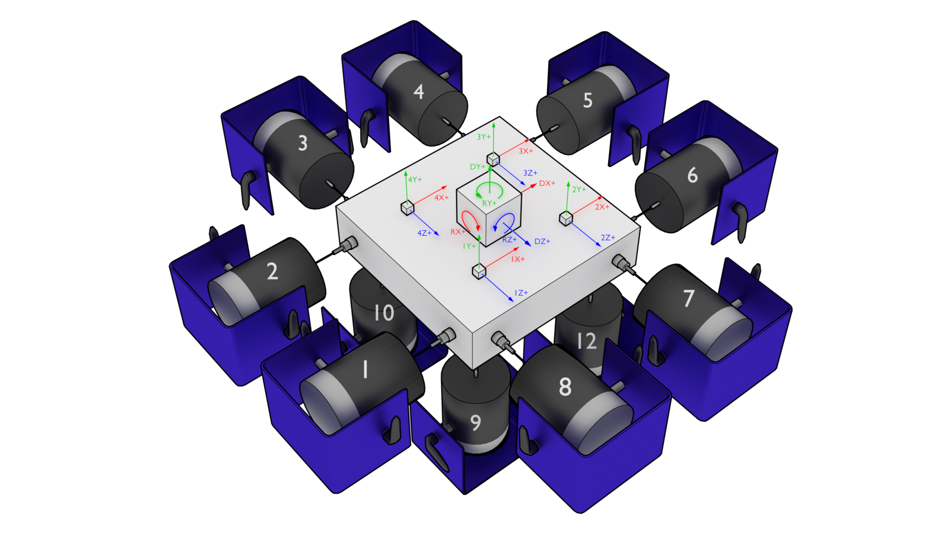
Figure 12.7:Representative 6DoF setup showing 12 shakers attached to a rigid table with four triaxial accelerometers measuring the table’s response. Note that shaker 11 is occluded by the table in this figure.
To set up the output transformation, one should examine the geometry of the test setup to identify which shakers excite which motions. For example, to move the table vertically in the Y+ direction, the four bottom shakers (9, 10, 11, and 12) should excite with a positive signal (here, a positive signal is assumed to be compressive, pushing the table away from the shaker; this may vary depending on shaker wiring). For this case, the row of the output transformation matrix should contain a 1 for shaker signals 9, 10, 11, and 12, and a zero for other shakers. Similar reasoning can be used for rotations: to rotate about the positive Z+ direction, shakers 11 and 12 should push with a positive signal and shakers 9 and 10 should pull with a negative signal. Therefore, the row corresponding to this degree of freedom would have -1 for shakers 9 and 10 and +1 for 11 and 12. The full output transformation for this case can be seen in Table 12.1. This matrix transforms the 12 physical shaker signals into 6 rigid body motions of the table.
Table 12.1:Output transformation for the 6DoF test shown in Figure 12.7
| Shaker | 1 | 2 | 3 | 4 | 5 | 6 | 7 | 8 | 9 | 10 | 11 | 12 |
|---|---|---|---|---|---|---|---|---|---|---|---|---|
| DX+ | 1 | 1 | 0 | 0 | -1 | -1 | 0 | 0 | 0 | 0 | 0 | 0 |
| DY+ | 0 | 0 | 0 | 0 | 0 | 0 | 0 | 0 | 1 | 1 | 1 | 1 |
| DZ+ | 0 | 0 | 1 | 1 | 0 | 0 | -1 | -1 | 0 | 0 | 0 | 0 |
| RX+ | 0 | 0 | 0 | 0 | 0 | 0 | 0 | 0 | -1 | 1 | 1 | -1 |
| RY+ | 1 | -1 | 1 | -1 | 1 | -1 | 1 | -1 | 0 | 0 | 0 | 0 |
| RZ+ | 0 | 0 | 0 | 0 | 0 | 0 | 0 | 0 | -1 | -1 | 1 | 1 |
To generate the response transformation matrix, it is often helpful to construct the inverse transformation and then invert it to recover the response transformation matrix. As an example, we will investigate the measured signals by the accelerometers if the table is translated one unit in the X+ direction. In this case, all accelerometers pointing in the X+ direction would see a one unit signal. Therefore the column of the inverse transformation corresponding to a X+ direction motion would have 1 for all channels pointing in that direction. If the table is rotated about the Y+ direction, the 1X+, 1Z+, 2X+, and 4Z+ channels will see positive motion, and the 2Z+, 3X+, 3Z+ and 4X+ channels will see negative motions, so the rows corresponding to those channels should be populated with +1 or -1, respectively. Note that there technically should be a moment arm computed by the distance from the accelerometer to the center-line of the table in the real rotation calculation; however, if all accelerometers are equidistant, this term can be dropped, and the system identification will compensate accordingly. Table 12.2 shows the constructed inverse transformation, and Table 12.3 shows the response transform matrix that should be provided to Rattlesnake.
Table 12.2:Inverse response transformation for the 6DoF test shown in Figure 12.7
| Channel | DX+ | DY+ | DZ+ | RX+ | RY+ | RZ+ |
|---|---|---|---|---|---|---|
| 1X+ | 1 | 0 | 0 | 0 | 1 | 0 |
| 1Y+ | 0 | 1 | 0 | -1 | 0 | -1 |
| 1Z+ | 0 | 0 | 1 | 0 | 1 | 0 |
| 2X+ | 1 | 0 | 0 | 0 | 1 | 0 |
| 2Y+ | 0 | 1 | 0 | -1 | 0 | 1 |
| 2Z+ | 0 | 0 | 1 | 0 | -1 | 0 |
| 3X+ | 1 | 0 | 0 | 0 | -1 | 0 |
| 3Y+ | 0 | 1 | 0 | 1 | 0 | 1 |
| 3Z+ | 0 | 0 | 1 | 0 | -1 | 0 |
| 4X+ | 1 | 0 | 0 | 0 | -1 | 0 |
| 4Y+ | 0 | 1 | 0 | 1 | 0 | -1 |
| 4Z+ | 0 | 0 | 1 | 0 | 1 | 0 |
Table 12.3:Response transformation for the 6DoF test shown in Figure 12.7
| Channel | 1X+ | 1Y+ | 1Z+ | 2X+ | 2Y+ | 2Z+ | 3X+ | 3Y+ | 3Z+ | 4X+ | 4Y+ | 4Z+ |
|---|---|---|---|---|---|---|---|---|---|---|---|---|
| DX+ | 0.250 | 0.000 | 0.000 | 0.250 | 0.000 | 0.000 | 0.250 | 0.000 | 0.000 | 0.250 | 0.000 | 0.000 |
| DY+ | 0.000 | 0.250 | 0.000 | 0.000 | 0.250 | 0.000 | 0.000 | 0.250 | 0.000 | 0.000 | 0.250 | 0.000 |
| DZ+ | 0.000 | 0.000 | 0.250 | 0.000 | 0.000 | 0.250 | 0.000 | 0.000 | 0.250 | 0.000 | 0.000 | 0.250 |
| RX+ | 0.000 | -0.250 | 0.000 | 0.000 | -0.250 | 0.000 | 0.000 | 0.250 | 0.000 | 0.000 | 0.250 | 0.000 |
| RY+ | 0.125 | -0.000 | 0.125 | 0.125 | 0.000 | -0.125 | -0.125 | -0.000 | -0.125 | -0.125 | -0.000 | 0.125 |
| RZ+ | -0.000 | -0.250 | -0.000 | 0.000 | 0.250 | -0.000 | 0.000 | 0.250 | 0.000 | 0.000 | -0.250 | 0.000 |
Note that when a response transformation matrix is used, the vibration specification must be delivered to Rattlesnake in terms of the transformed coordinates. Note that the specification in terms of physical measurement can be transformed into the virtual quantities in the same way that the physical quantities themselves are transformed.
Transformation matrices can be used for more general coordinate system transformations. Perhaps the vibration specification has been derived from a finite element model, but the test article has instrumentation mounted obliquely to the global finite element coordinate system. A transformation matrix consisting a rotation matrices can be used to transform between coordinate systems in the model and coordinate systems in the test. Additionally, transformation matrices can be used to perform spatial filtering for example to control to specific modes of the structure . Given the modal transformation
the modal quantities can be computed from physical quantities as
In this case, the transformation matrix is simply the inverse mode shape matrix , which acts as a modal filter.
12.8.1Specifying Transformation Matrices
Transformation matrices are specified by clicking the Transformation Matrices... button, which will bring up a dialog box allowing users to define the transformations. This is shown in Figure 12.8.
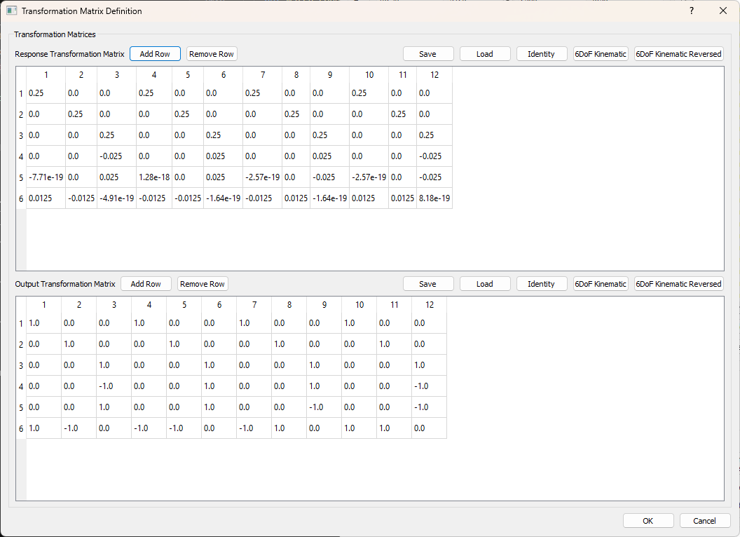
Figure 12.8:Transformation Matrix Dialog Box
The top portion of the window corresponds to the Response Transformations, which are transformations applied to the physical control channels to create virtual control channels, and the bottom portion of the window corresponds to the Output transformations, which are transformations applied to the physical excitation channels to create virtual excitation sources.
The number of rows in each matrix are the number of virtual channels that exist in the environment. Virtual channels can be added or removed by adding or removing rows of the matrices. The number of columns in each matrix corresponds to the number of physical channels that exist in the environment. The number of columns is therefore specified by the number of control or excitation degrees of freedom active in the environment; these cannot be changed in the Transformation Matrix Definition dialog box, but must rather be changed through the channel table or environment definition.
To remove transformations, the matrices can simply be set to the identity matrix, in which case, each physical degree of freedom corresponds directly to a virtual degree of freedom, meaning the virtual degrees of freedom are the physical degrees of freedom.
Rather than entering the matrix values manually, which may be tedious for a large test, users can load transformation matrix from CSV, *.mat, *.npy, or *.npz files. Users can also save existing transformation matrices to those file types.
Response Transformation Matrix Add Row Add a virtual control channel to the response transformation
Response Transformation Matrix Remove Row Remove the selected virtual control channel from the response transformation
Response Transformation Matrix Save Opens a file dialog allowing the user to save the response transformation matrix to a file.
Response Transformation Matrix Load Opens a file dialog to allow the user to load in a response transformation matrix from a file.
Response Transformation Matrix Identity Set the response transformation to the identity matrix (effectively removes the transformation)
Response Transformation 6DoF Kinematic Sets the response transformation matrix to a kinematic transformation matrix based on a typical 6-DoF shaker configuration, such as that found in the Team Tensor shaker.
Response Transformation 6DoF Kinematic Reversed Sets the response transformation matrix to a kinematic transformation matrix based on a typical 6-DoF shaker configuration, such as that found in the Team Tensor shaker. This default switches the signs on some of the coefficients based on shaker wiring.
Output Transformation Matrix Add Row Add a virtual excitation channel to the output transformation
Output Transformation Matrix Remove Row Remove the selected virtual excitation channel from the output transformation
Output Transformation Matrix Save Opens a file dialog allowing the user to save the output transformation matrix to a file.
Output Transformation Matrix Load Opens a file dialog to allow the user to load in an output transformation matrix from a file.
Output Transformation Matrix Identity Set the output transformation to the identity matrix (effectively removes the transformation)
Output Transformation 6DoF Kinematic Sets the output transformation matrix to a kinematic transformation matrix based on a typical 6-DoF shaker configuration, such as that found in the Team Tensor shaker.
Output Transformation 6DoF Kinematic Reversed Sets the output transformation matrix to a kinematic transformation matrix based on a typical 6-DoF shaker configuration, such as that found in the Team Tensor shaker. This default switches the signs on some of the coefficients based on shaker wiring.
To exit the dialog, the user will press either the OK button to keep the specified transformations, or the Cancel dialog to reject the specified transformations.
OK Saves the transformation matrices to the environment
Cancel Cancels modification of the transformation matrices
12.9Generation of Time Histories
Rattlesnake’s MIMO Random Vibration environment allows users to run custom control laws that produce CPSD matrices. Rattlesnake must then create time histories from those CPSD matrices to send to the shakers. This section will discuss some of the implementation details of this process that may be useful for users to understand.
12.9.1Creating Time Signal Realizations from CPSD Matrices
To start the signal generation process, the signal generation routine receives an output CPSD matrix from the custom control law provided by the user. The controller uses the process described in 3 to create a time history realization from the CPSD matrix. Note that for large control problems, it might take more than one measurement frame to perform the control problem, so there might not be an output CPSD matrix ready when the controller requires it. In that case, the previous output CPSD matrix is used.
To generate a time history realization, the square root of the CPSD matrix is taken using a SVD approach. This creates linear spectra from the power spectra.
A random process vector is computed using Gaussian real and imaginary components and .
where is the frequency spacing and is the complex variable.
A realization of the linear spectra is computed by multiplying the random process vector by the linear spectra
Taking the inverse FFT then transforms the linear spectra into time signals that can be sent to the shakers.
Note that this signal has the length of one FFT frame, which is generally not long enough to be immediately useful for vibration testing. Multiple signals can be generated by taking additional realizations of the random process vector; however, simply concatenating multiple realizations will result in discontinuous signals, as there is no guarantee that these signals will start and end at the same levels.
12.9.2Synthesizing Continuous Time Histories using COLA
To handle the synthesis of longer signals, a COLA process is used. This process is also described in detail in 3. A COLA window function is specified that allows each time history realization to start and end at zero. To ensure the proper variance is maintained, the square root of the window function is applied to the signal (specified using the Window Exponent parameter in the Environment Definition tab). The overlap is specified such that the original (un-square-rooted) window function sums to one over the signal. The windowed signals are then added together to form a continuous signal.
Rattlesnake cannot realistically compute a large number of realizations all at once to create one long signal, as this would impede its ability to respond to changing test conditions, effectively making it an open-loop control system. Instead, Rattlesnake must compute this COLA operation on the fly. It does this by keeping two output signals in memory at once. It overlaps the last part of the first signal with the first part of the next signal and sends that overlapped portion of the signal to the output of the controller. Then, the previous next signal becomes the next first signal and a new realization replaces the previous next signal and the process continues.
12.9.3Setting the Test Level
The final operation performed on the output signal is to adjust for test level. Initial versions of the Rattlesnake simply scaled the vibration specification so the controller would naturally scale its output to match the scaled specification. This was found to be lacking especially for large control problems where it could take a second or more to perform a control calculation. This combined with the COLA approach meant that it could take several seconds for a test level change to be realized, which was more than enough time to damage test hardware. Another issue with this approach was for error-based control approaches. The controller would immediately recognize that it was in error due to the change in test level and produce a modified output. However, there could be 20 or more frames of data being used in the computation of CPSD matrices that would need to be overwritten prior to the controller recovering. In practice, this meant that the controller would severely overshoot the desired level as it further and further modified the output with very little change in the response CPSD. One final issue is that it relied on the COLA process to smooth jumps between test levels. As the COLA overlap regions could be quite short, this lead to fairly severe level changes that could damage test hardware.
Recent versions of the Rattlesnake have moved away from scaling the vibration specification and started scaling the output signal directly. The acquired data is then scaled back to full level prior to control calculations taking place. For this reason, all information written to the Run Test tab in the GUI is presented as if it were at full level. Because the time histories are modified directly, it allows ramping between test levels to be implemented directly and at whatever speed is required for hardware safety. Data acquired during the ramp between test levels is generally ignored; only data acquired while the test level is constant is used for spectral computations.
- Schultz, R., & Avitabile, P. (2020). Shape-constrained Input Estimation for Efficient Multi-shaker Vibration Testing. Experimental Techniques, 44(4), 409–423. 10.1007/s40799-020-00361-0
- Daborn, P. M. (2014). Smarter dynamic testing of critical structures [Phdthesis]. University of Bristol.
- Schultz, R. A., & Nelson, G. D. (2020). Input Signal Synthesis for Open-Loop Multiple-Input/Multiple-Output Testing. In C. Walber, P. Walter, & S. Seidlitz (Eds.), Sensors and Instrumentation, Aircraft/Aerospace, Energy Harvesting and Dynamic Environments Testing, Volume 7 (pp. 245–257). Springer International Publishing.