Burgers Example#
This example builds a reduced-order model for 1D Burgers’ equation, trains a structure-preserving NN-OpInf model, and compares it against a baseline unstructured model.
Run it:
python examples/burgers/burgers_end_to_end.py
Key outputs:
Plot:
examples/burgers/burgers_solution.pdfTrained models:
examples/burgers/ml-models/
Code#
import numpy as np
from matplotlib import pyplot as plt
import yaml
import argparse
import sys
import nnopinf
import nnopinf.operators as operators
import nnopinf.models as models
import nnopinf.training
import torch
from matplotlib import pyplot as plt
axis_font = {'size':'20'}


def upwind_deriv(u,dx):
  r = np.zeros(u.size)
  fsym = np.zeros(u.size)
  fsym[0] = 1./6.*(u[0]**2 + u[0]*u[-1] + u[-1]**2)
  fsym[1::] = 1./6.*(u[1::]**2 + u[1::]*u[0:-1] + u[0:-1]**2)

  lamRoe = np.zeros(u.size)
  du = np.zeros(u.size)

  lamRoe[1::] = 0.5*np.abs(u[1::] + u[0:-1])
  lamRoe[0] = 0.5*np.abs(u[0] + u[-1])

  du[1::] = (u[1::] - u[0:-1])
  du[0] = (u[0] - u[-1])

  fL = np.zeros(u.size)
  fL[:] = fsym[:] - 0.5*(lamRoe + np.abs(du)/6.)*du
  fR = np.roll(fL,-1)
  r = fR - fL
  return r/dx

class burgers_fom:
  def __init__(self,L,nx):
    self.L = L
    self.N = nx
    self.nx = nx
    self.dx = self.L / self.N

    self.x = np.linspace(0,self.L - self.dx,self.nx)
    self.u0 = np.sin(self.x)

  def velocity(self,u):
    f = -upwind_deriv(u,self.dx)
    return f


  def solve(self,dt,end_time):
    u = self.u0
    t = 0.
    rk4const = np.array([1./4.,1./3.,1./2.,1.])
    u_snapshots = np.zeros((self.nx,0))
    f_snapshots = np.zeros((self.nx,0))
    counter = 0
    t_snapshots = np.zeros(0)
    while t <= end_time - dt/2.:
      u_snapshots = np.append(u_snapshots,u[:,None],axis=1)
      t_snapshots = np.append(t_snapshots,t)

      u0 = u*1.
      for i in range(0,4):
        f = self.velocity(u)
        u = u0 + dt*rk4const[i]*f
      t += dt
      counter += 1
    return u_snapshots,t_snapshots


class nn_opinf_rom:
  def __init__(self,model):
    self.model_ = model
    self.inputs_ = {}
  def velocity(self,u):
    self.inputs_['x'] = torch.tensor(u[None])

    ft = self.model_.forward(self.inputs_)[0].detach().numpy()
    return ft


  def solve(self,u0,dt,end_time):
    u = u0
    t = 0.
    rk4const = np.array([1./4.,1./3.,1./2.,1.])
    u_snapshots = np.zeros((u0.size,0))
    f_snapshots = np.zeros((u0.size,0))
    counter = 0
    t_snapshots = np.zeros(0)
    while t <= end_time - dt/2.:
      u_snapshots = np.append(u_snapshots,u[:,None],axis=1)
      t_snapshots = np.append(t_snapshots,t)

      u0 = u*1.
      for i in range(0,4):
        f = self.velocity(u)
        u = u0 + dt*rk4const[i]*f
      t += dt
      counter += 1
    return u_snapshots,t_snapshots


if __name__=='__main__':

    ## Setup and solve the FOM
    nx = 500
    L = 2.*np.pi
    myFom = burgers_fom(L,nx)
    dt = 0.01
    et = 5.
    u,t = myFom.solve(dt,et)

    # Make POD basis
    Phi,s,_ = np.linalg.svd(u,full_matrices=False)
    relative_energy = np.cumsum(s**2) / np.sum(s**2)
    K = 10#np.argmin(np.abs(relative_energy - 0.99999999))
    Phi = Phi[:,0:K]

    #Now do nnopinf
    uhat = Phi.transpose() @ u
    uhat_dot = (uhat[:,2::] - uhat[:,0:-2]) / (2.*dt)
    # Trim to make the same size
    uhat = uhat[...,1:-1]

    # Design operators
    n_hidden_layers = 5
    n_neurons_per_layer = K
    n_inputs = K
    n_outputs = K

    # Design operators for the state.
    # Create to be energy conserving , s.t. uhat_dot \le 0
    x_input = nnopinf.variables.Variable(size=K,name='x',normalization_strategy='MaxAbs')
    target = nnopinf.variables.Variable(size=K,name='y',normalization_strategy='MaxAbs')

    NpdMlp = nnopinf.operators.SpdOperator(acts_on=x_input,depends_on=(x_input,),n_hidden_layers=n_hidden_layers,n_neurons_per_layer=n_neurons_per_layer,positive=False)
    SkewMlp = nnopinf.operators.SkewOperator(acts_on=x_input,depends_on=(x_input,),n_hidden_layers=n_hidden_layers,n_neurons_per_layer=n_neurons_per_layer)

    # Create a model using the two operators
    pd_model = nnopinf.models.Model( [NpdMlp,SkewMlp] )

    # Train
    training_settings = nnopinf.training.get_default_settings()
    training_settings['batch-size'] = 500
    training_settings['num-epochs'] = 10000
    training_settings['GN-final-layer'] = True
    training_settings['GN-num-layers'] = 1
    training_settings['LBFGS-acceleration'] = False
    training_settings['GN-final-layer-damping'] = 0
    training_settings['GN-final-layer-epoch-frequency'] = 25
    print("Settings are: ",training_settings)

    x_input.set_data(uhat.transpose())
    target.set_data(uhat_dot.transpose())

    variables = [x_input]
    print('Training Positive Definite Model')
    nnopinf.training.trainers.train(pd_model,variables=variables,y=target,training_settings=training_settings)

    # Compare to the basic approach
    BasicMlp = nnopinf.operators.StandardOperator(n_outputs=K,depends_on=(x_input,),n_hidden_layers=n_hidden_layers,n_neurons_per_layer=n_neurons_per_layer)
    basic_model = nnopinf.models.Model( [BasicMlp] )
    print('Training Basic Model')
    nnopinf.training.trainers.train(basic_model,variables=variables,y=target,training_settings=training_settings)


    # Do a forward pass of both models
    u0 = Phi.transpose() @ myFom.u0
    pd_rom = nn_opinf_rom(pd_model)
    u_pdrom,t_ndrom = pd_rom.solve(u0,dt,et)
    u_pdrom = Phi @ u_pdrom

    basic_rom = nn_opinf_rom(basic_model)
    u_basicrom,t_basicrom = basic_rom.solve(u0,dt,et)
    u_basicrom = Phi @ u_basicrom

    # Check errors and plot
    relative_error = np.linalg.norm(u_pdrom - u)/np.linalg.norm(u)
    print('ND ROM relative error = ' + str(relative_error))
    relative_error = np.linalg.norm(u_basicrom - u)/np.linalg.norm(u)
    print('Basic ROM relative error = ' + str(relative_error))

    plt.close("all")
    plt.plot(myFom.x,u[:,-1],color='black',label='FOM')
    plt.plot(myFom.x,u_pdrom[:,-1],'--',color='blue',label='NNOPINF (Positive Definite)')
    plt.plot(myFom.x,u_basicrom[:,-1],'--',color='green',label='NNOPINF (No structure)')
    plt.xlabel(r'$x$',**axis_font)
    plt.ylabel(r'$u(x)$',**axis_font)
    plt.legend()
    plt.tight_layout()
    plt.savefig('burgers_solution.pdf')
Walkthrough#
Generate full-order snapshots. The script solves Burgers’ equation with a finite-volume upwind flux and RK4 time stepping, storing state snapshots over time.
Build a reduced basis. It performs an SVD on the snapshots and truncates to retain almost all energy, yielding a low-dimensional basis
Phi.Project to reduced coordinates. It projects snapshots into the reduced space and estimates time derivatives with centered differences.
Define NN-OpInf operators. It constructs a positive-definite operator and a skew-symmetric operator to enforce energy structure, then wraps them into a model.
Train the model. It normalizes data, optimizes network weights, and saves the trained operators and the composite model.
Baseline comparison. It trains a standard (unstructured) operator model on the same data.
Evaluate and plot. It integrates the learned ROMs forward in time and compares the final state against the full-order model.
Final plot#
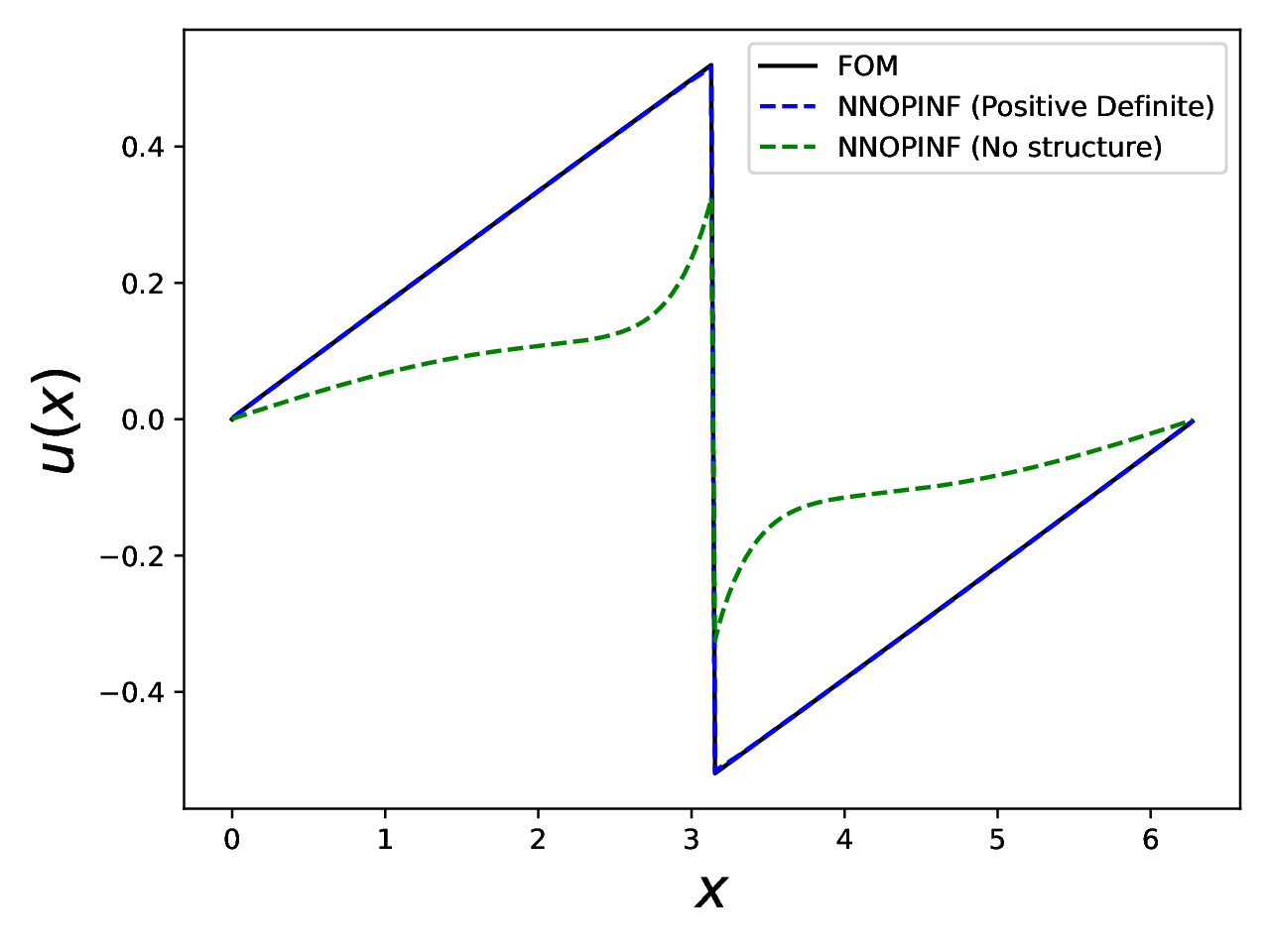
Burgers’ equation: full-order solution vs. NN-OpInf ROMs at the final time.#
Tips#
The script uses a long training horizon. For a quick smoke test, lower
num-epochsand increasebatch-sizenear the top of the script.Output PDFs are written in the example directory.